Journal of Mathematical Finance
Vol.06 No.04(2016), Article ID:71178,21 pages
10.4236/jmf.2016.64042
Calibration and Simulation of Arbitrage Effects in a Non-Equilibrium Quantum Black-Scholes Model by Using Semi-Classical Methods
Mauricio Contreras, Rely Pellicer, Daniel Santiagos, Marcelo Villena
Facultad de Ingeniería y Ciencias, Universidad Adolfo Ibáñez, Santiago, Chile

Copyright © 2016 by authors and Scientific Research Publishing Inc.
This work is licensed under the Creative Commons Attribution International License (CC BY 4.0).
http://creativecommons.org/licenses/by/4.0/


Received: August 23, 2016; Accepted: October 9, 2016; Published: October 12, 2016
ABSTRACT
An non-equilibrium Black-Scholes model, where the usual constant interest rate r is replaced by a stochastic time dependent rate r(t) of the form , accounting for market imperfections and prices non-alignment, is developed. The white noise amplitude
 , called arbitrage bubble, generates a time dependent potential
  which changes the usual equilibrium dynamics of the traditional Black-Scholes model. The purpose of this article is to tackle the inverse problem, that is, is it possible to extract the time dependent potential
  and its associated bubble shape
  from the real empirical financial data? In order to give an answer to this question, the interacting Black-Scholes equation must be interpreted as a quantum Schrödinger equation with Hamiltonian operator
 , where
  is the equilibrium Black-Scholes Hamiltonian and
  is the inter- action term. By using semi-classical considerations and the knowledge about the mispricing of the financial data, one can determinate an approximate functional form of the potential term
  and its associated bubble
 . In all the studied cases, the non-equilibrium model performs a better estimation of the real data than the usual equilibrium model. It is expected that this new and simple methodology could help to improve option pricing estimations.
Keywords:
Option Pricing, Non-Equilibrium Black-Scholes Model, Semi-Classical Approximation, Quantum Mechanical Methods, Crank-Nicholson Method

1. Introduction
For almost 35 years, since the seminal articles by Black and Scholes [1] and Merton [2] , the Black-Scholes (B-S) model has been widely used in financial engineering to model the price of a derivative on equity. In analytic terms, if  and
and  are the risk- free asset and underlying stock prices, the price dynamics of the bond and the stock in this model are given by the following equations:
 (1)
(1)
where ,
,  and
and  are constants and
  is a Wiener process. In order to price the financial derivative, it is assumed that it can be traded, so one can form a portfolio based on the derivative and the underlying stock (no bonds are included). Considering only non-dividend paying assets and no consumption portfolios, the purchase of a new portfolio must be financed only by selling from the current portfolio. Here,
  denotes the option price,
  is the portfolio and
  is the price vector of shares. Calling
  the value of the portfolio at time t, the dynamic of a self-financing portfolio with no consumption is given by
 . (2)
. (2)
In other words, in a model without exogenous incomes or withdrawals, any change of value is due to changes in asset prices.
Another important assumption for deriving B-S equation is that the market is efficient in the sense that is free from arbitrage possibilities. This is equivalent with the fact that there exists a self-financed portfolio with value process  satisfying the dynamic:
 (3)
(3)
which means that any locally riskless portfolio has the same rate of return than the bond.
For the classical model presented above, there exists a well known solution for the price process of the derivative  (see, for example [3] ). Given its simplicity, this formulation can be described as one of the most popular standards in the profession.
Today however, it is possible to find models that have relaxed almost all of the initial assumptions of the Black-Scholes model, such as models with transaction costs, different probability distribution functions, stochastic volatility, imperfect information, etc.; all of which have improved the prediction capabilities of the original B-S model (see [3] - [6] for some complete reviews of these extensions).
Some attempts to improve the predictions of the Black-Scholes models, which take into account deviations of the equilibrium in the form of arbitrage situations, have been developed in [7] - [11] . In this case, some of these models assume that the return from the B-S portfolio is not equal to the constant risk-free interest rate, but instead, the no arbitrage principle (3) is modified according to the equation
 (4)
(4)
where  is a random arbitrage return. This formulation gives great flexibility to the model, since
  can be seen as any deviations of the traditional assumed equi- librium, and not just as an arbitrage return. For instance, Ilinski [12] and Ilinski and Stepanenko [13] assume that
  follows an Ornstein-Uhlenbeck process. Deviation from the non-arbitrage assumption implies that investors can make profit in excess from the risk-free interest rate. For example, if
  is greater than zero, then what one can do is: borrow from the bank, paying interest rate r, invest in the risk-free rate stock portfolio and make a profit. Alternatively, one could go short the option, delta hedging it.
The object of this paper, is to study the arbitrage effects on the option prices. This study will have two principal components:
1) Calibration: hopes to obtain a measure of the arbitrage effects from the empirical financial data, and
2) Simulation: the above measure can be used to obtain the “improved” option price and compare it with the usual Black-Scholes model and the real option prices.
For this, it is assumed that arbitrage can be modelled using Equation (4), so it will consider the B-S model in (1) and self-financing portfolio condition in (2) and in what follows the following arbitrage condition is assumed:
 (5)
(5)
where  is a given deterministic function called “arbitrage bubble” [7] and W is the same Wiener process in the dynamic of the underlying stock S. Equation (5) will generate a non-equilibrium Black-Scholes model. Note that condition (5) can be rewritten as
 (6)
(6)
where  is a white noise. This can be interpreted as a stochastic perturbation in the rate of return of the portfolio with amplitude f:
 .
.
As it is well known, in a perfectly competitive market, assumed by the original B-S model, the action of buyers and sellers exploiting the arbitrage opportunity will cause the elimination of the arbitrage in the very short run, so in our setting one will considered implicitly the speed of market’s adjustment by modelling an “arbitrage bubble”, which can be defined in duration and size, taking this way into account the market clearance power. All this information is contained in the function . In fact, in [7] it is shown that, for an infinite arbitrage bubble f the non equilibrium Black-Scholes model goes to the usual Black-Scholes model, so (5) accounts implicitly for the market power clearance.
In [9] - [13] different generalizations of the Black-Scholes model are proposed. These models include a stochastic rate model whose dynamic is generated by a second Brownian motion independent of the asset Brownian motion. In a sense, these models are inspired by “stochastic volatility ideas”.
What it is done here, is to incorporate arbitrage effects, but as close as possible to the original Black-Scholes model, which has only one source of randomness (associated with the asset price S) and where the B bonus dynamics is completely deterministic.
The central idea is that arbitrage effect can change the portfolio returns in a random fashion, and the source of randomness must be generated by the same asset Brownian motion. It is in that sense that the term “endogenous stochastic arbitrage” appears in the title of paper [7] . In that setting, the only remaining degree of freedom necessary is the amplitude of such a Brownian motion that is expressed in Equation (5).
Although, Equation (5) can be rewritten as a stochastic rate model as in Equation (6), it is not clear if such interpretation is well defined in mathematical terms, or if even it is integrable. So, the point of view taken here is not to see the model as a stochastic rate model, but instead as a “perturbed portfolio return model”, defined by Equation (5).

1Otherwise, the arbitrage should be modelled exogenously to the B-S model.
Thus, it is assumed a model-dependent arbitrage, where the arbitrage possibilities are modelled with the same stochastic process that govern the underlying stock. This assumption allows to link the arbitrage equation to the B-S original model1 This assumption is reasonable from a theoretical perspective for some kinds of arbitrages, which are inherent to the underlying asset, and endogenous in nature to the asset in analysis. The validity of this maintained hypothesis has been tested empirically, for example in [14] .
In [7] analytical solutions of the non equilibrium Black-Scholes model were found for a time dependent “step function” arbitrage bubble f for an option with maturity T:
 . (7)
. (7)
This particular shape of the bubble was motivated by an empirical study of futures on the S&P 500 index between September 1997 and June 2009. There, through the empirical analysis of the future mispricing, one can get the shape of the arbitrage bubble, which in that case corresponds roughly to a step function shape, as is showed in Figure 1.
So in the option pricing context, it can be naturally asked: can the shape of the

Figure 1. Future’s mispricing.
arbitrage bubble f be obtained from an empirical analysis of the option mispricing, using the same approach for futures on the S&P 500 index given in [7] ?
The object of this paper is to show that the answer is positive and to develop a methodology for extracting the arbitrage bubble f from the empirical financial data through the analysis of the option mispricing. In order to do that, it will be needed to use some results of semi-classical approximations applied to option pricing as develop in [8] . There, an approximate solution for the non equilibrium Black-Scholes equation in the presence of an arbitrary arbitrage bubble was constructed. This semi-classical solution with the option mispricing data, permit to obtain a non linear equation for the arbitrage bubble. By solving this equation by means of numerical methods the approximate shape of the arbitrage bubble f can be obtained. Then, taking this arbitrage bubble back to the non equilibrium Black-Scholes equation, it can be determined the “exact” interacting option price solution by means of a Crank-Nicolson method and compare it with the usual equilibrium Black-Scholes solution. In all studied cases, the non equilibrium solution performs a better numerical estimation for the empirical data than the usual Black-Scholes solution.
To proceed and to make the paper self contained, section 2 reviews the interacting Black-Scholes model according to [7] and section 3 gives it interpretation as a quantum model. The section 4, quickly reviews the main results of semi-classical quantum ideas applied to the interacting Black-Scholes model as developed in [8] . In section 5, the calibration problem is analyzed, that is, how to estimate the interaction potential in the non-equilibrium Black-Scholes framework, and the deduction of an equation which permits to found arbitrage bubble  from the actual financial data.
In section 6, the simulation problem is developed to obtain the exact option price solution of the non-equilibrium model, for several different data sets. In section 7, final conclusion and future prospects are given.
2. The Non-Equilibrium Black-Scholes Model
Following [7] , the price dynamics of the financial derivative under the endogenous arbitrage condition (5) is found. The price dynamic as the solution  of certain boundary value problem is derived. In what follows, the price process is considered depending on t, S, but this dependence is omitted for the sake of simplicity. Using Itö calculus:
 . (8)
. (8)
Given the dynamic for S in (1):
 . (9)
. (9)
Self-financing portfolio condition in (2) can be understood as . Considering this and (5) together and replacing dynamics for S and
 :
:
 (10)
(10)
Collecting dt- and dW-terms:
 (11)
(11)
The condition for existence of non-trivial portfolios  satisfying (11) gives that, given the B-S model for a financial market in (1), self-financing portfolio con- dition (2) and stochastic arbitrage condition in (5), the price process
  of the derivative is the solution of the following boundary value problem in the domain
 .
.
 (12)
(12)
for constant ,
,  ,
,  , any function f and a simple contingent claim
 .
.
Thus, Equation (12) shows a particular type of arbitrage, that occurs when the underlying asset and its arbitrage possibilities are generated by a common and endogenous stochastic process. This formulation is fairly general, in the sense that f could take any functional form. This function f will be called the arbitrage bubble. Note that when , the standard equilibrium B-S model is recovered.
It is important to stress here that the model generated by Equation (12) is an out- of-equilibrium model, in the sense that, it does not satisfies the martingale hypothesis for .
.
3. The Interacting Black-Scholes Model as a Schrödinger Quantum Equation
In this section, the Black-Scholes equation is interpreted as a Schrödinger wave equation and its consequences are explored. Significant attempts to see the Black-Scholes equation as quantum models can be found in [8] [14] - [17] . In this case, the Black- Scholes equation in the presence of an arbitrage bubble (12) can be written as
 (13)
(13)
where
 (14)
(14)
is the usual arbitrage free Black-Scholes operator. The factor
 (15)
(15)
can be interpreted as an effective potential induced by the arbitrage bubble . In this way, the presence of arbitrage generates an external time dependent force, which have an associated potential
 . Then the interacting Black-Scholes model developed in [7] corresponds, from a physics point of view, to an interacting particle with an external field force. Obviously, when arbitrage disappear, the external potential is zero and the usual Black-Scholes dynamics is recovered. One can also see that the option price dynamics
  depends explicitly on the arbitrage bubble form
 . From a financial optics, the arbitrage bubbles should be time-finite lapse and they should have a characteristic amplitude. So, in general, arbitrage bubbles can be defined by three parameters: the born-time, dead-time and the maximum amplitude between these two times. In [8] an approximate analytical solution for the non-equilibrium Black-Scholes equation, for an arbitrary arbitrage bubble form was found.
3.1. The Quantum Hamiltonian
Following [8] , where a Black-Scholes-Schrödinger model based on the endogenous arbitrage option pricing formulation introduced by [7] was developed, consider again the interacting Black-Scholes Equation (12) and take the variable change , to obtain
 (16)
(16)
making a second (time dependent) change of variables  holds
holds
 (17)
(17)
where
 . (18)
Now it is stated: Given the non equilibrium Black-Scholes model in (12) for the price of an option with arbitrage, and defining
 (19)
(19)
the  dynamics is given by
 (20)
(20)
where
 (21)
(21)
is the interaction potential in the  space.
The last two equations can be interpreted as a Schrödinger equation in imaginary time for a particle of mass  with wave function
  in an external time dependent field force generated by
 . Writing Schrödinger equation as
 (22)
(22)
and following the arguments developed by Baaquie in [18] the hamiltonian operator can be read as
 . (23)
Since momentum operator in imaginary time is
 (24)
(24)
finally the quantum hamiltonian for the interactive Black-Scholes model is derived as a function of the momentum operator.
 . (25)
3.2. The Underlying Classical Mechanics
In order to obtain a semi-classical approximation for the solution of the non-equili- brium Black-Scholes model, the classical equation of motion is developed, that is, the Newton equations associated to the quantum model. So, taking the classical limit  the quantum hamiltonian becomes the classical hamiltonian function
 . (26)
The classical hamiltonian equations
 (27)
(27)
reduces in this case to
 (28)
(28)
 . (29)
The corresponding lagrangian
 (30)
(30)
becomes
 . (31)
The Euler-Lagrange equation
 (32)
(32)
gives for this system, the following Newton equation
 . (33)
Some special cases are considered here in detail.
3.3. The Time-Independent Arbitrage Model
First, if the bubble depends only on S, that is , this imply that
 (34)
(34)
and in this case
 (35)
(35)
so the Newton equation reads
 (36)
(36)
or
 (37)
(37)
where
 . (38)
3.4. The Time-Dependent Arbitrage Model
In the second case, the arbitrage bubble depends only on time coordinate  so
so
 (39)
(39)
and
 (40)
(40)
so
 . (41)
The Euler-Lagrange equation reads now
 (42)
(42)
that is
 (43)
(43)
which can be easily integrated as
 (44)
(44)
where C and D are arbitrary constants.
In that follows, arbitrage bubbles that are time dependent are only considered, that is,
 . (45)
The reasons to do that are:
1) the model is more “simple” in mathematical terms and
2) the financial data available is time dependent but no S dependent.
In a further study the behaviour of the interacting Black-Scholes model is analyzed for arbitrage bubbles that depends explicitly on the underlying asset price S.
Note that for the time dependent arbitrage bubble , the
, the  potential in (15) and the
  potential in (21) are completely equivalent:
 .
.
4. Path Integrals and the Semi-Classical Approximation
Path integrals and semi-classical methods have been used to find approximate solutions of the Schrödinger equation in different areas of theoretical physics, such as nuclear physics [19] , quantum gravity [20] , chemical reactions [21] , quantum field theory [22] and stochastic processes [23] . Path integrals also have been used to price the value of an option, for example see [8] [18] [24] - [30] . In this section, the semi-classical approxi- mation is applied to found an approximate solution for the option price.
It is well known that when a system has interactions, the semi-classical approach gives an approximate solution for the wave function of the system, while for free interaction case, semi-classical approximation can give exact results [31] . In this section, following [8] a financial application is developed, based on the quantum arbitrage model of the previous section.
In a general setting, the solution of the Schrödinger Equation (22) can be written as
 (46)
(46)
where  is a specific contract (Call, Put, Binary Call…) in the x space, and
  is the propagator which admits the path integral representation
 (47)
(47)
where  is the classical action evaluated over the path
 (
( ) and the integral is done over all paths that connect the points
  and
and . If one writes
  as
as  and expands the action around the classical path, one has
 (48)
(48)
(where all functional derivatives are evaluated on the classical path ) and integrate over all trajectories
 , the propagator becomes
 . (49)
Considering contributions up to second order terms (see for example [23] ), the semi- classical approximation for the propagator G is given by
 . (50)
On the other hand, the solution for the option price  in the
  space is then
 (51)
(51)
so the propagator for the option price is, in the semi-classical approximation
 . (52)
In order to found the semi-classical approximation for the option price, in presence of a time dependent arbitrage bubble , the classical solution (44) for a time variable
  (
( ) must be obtained first, with the initial condition
  and final condition
 . This implies that the constant C in (44) is given by
 (53)
(53)
so the Lagrangian (31) evaluated over the classical path is
 (54)
(54)
and the action  evaluated over the classical path becomes
finally
 (55)
(55)
where
 (56)
(56)
is the accumulative potential between t and T.
The semi-classical propagator in the x space is then according to (52)
 . (57)
By using the transformation
 (58)
(58)
and the fact that , one can now writes the semi-classical propagator in the
  space as
 (59)
(59)
so the semi-classical solution for the option price is then given by
 . (60)
Now, note that the Black-Scholes propagator is just the semi-classical propagator (59) evaluated at 
 (61)
(61)
so the pure Black-Scholes solution is
 . (62)
From (59) and (61) one can see that both propagators are related by
 (63)
(63)
and from (60)
 (64)
(64)
which due to (62), is equivalent to say
 . (65)
The last equation therefore, is the semi-classical approximation for the non equilibrium Black-Scholes solution for the option price, in presence of an arbitrary time dependent arbitrage bubble . Here
  is the arbitrage-free Black-Scholes solution for the specific option with contract
  and
and  is the accumulative potential given by (56).
In this way, the function  renormalizes the bare arbitrage-free Black-Scholes solution. One important fact of this last equation is that it permits to obtain an appro- ximation of our Black-Scholes-Schrödinger interacting model from the classical Black- Scholes model, by means of a rescaling of the price variable, so usual computational codes can be easily modified to obtain an approximation for the interacting model.
5. Interaction Potential and Arbitrage Bubble Calibration
Now finally, after a long trip on the interacting model and its semi-classical approxi- mation, the main two point of this paper can be tackled, that is, the calibration and simulation problem for the arbitrage bubble and for the option price solution of the non equilibrium Black-Scholes model respectively.
In order to solve the calibration problem, consider the empirical time-series of the underlying asset  and the real price of the option
  in the interval
 . One can ask for the interaction potential function
 (66)
(66)
associated to a time dependent arbitrage bubble  that allows the solution
  of Equation (13) when evaluated over
  to fit all the time-serie of
 .
.
One way to proceed is to take a definite functional form for the U function with parameters . In this case the solution of (6) becomes a function of the vector
  and then, the set of coefficients
  can be determined minimizing the quantity
 (67)
(67)
over all sets of coefficients . But it is not clear if such a minimum exists or there exist several local minima and the problem reduces to find the true one. Numerically this problem can turn to be impossible to achieve. Moreover, initial guess for U is a matter of taste, and it is not clear what the correct initial functional form is and from which the
  minimization can start.
In order to determine a guess function for the U potential a different path has to be follow, based on the semi-classical approximation and the notion of mispricing. The mispricing, denoted by , is defined in [32] as the difference between the empirical option price
  and the value of Black-Scholes solution
  evaluated over the empirical underlying asset price
 . (68)
Naturally, the function  above is known only over a discrete time set of points. Let
  be the exact potential originated by the exact arbitrage bubble
  which gives the correct empirical option price when the solution of the interacting Black- Scholes model (13)
  is evaluated over the empirical underlying asset price
 (69)
(69)
the solution  makes the value of the Equation (67) be exactly zero. Now suppose that
  potential is weak (
 ), in such a way that the semi-classical approxi- mation for the option price is valid, so the option price
  can be replaced by its semi-classical approximation (65)
 (70)
(70)
where
 (71)
(71)
so the mispricing Equation (68) becomes an equation for the arbitrage bubble 
 . (72)
Equation (72) is the most important equation of this paper, because it allows, from the knowledge about the empirical mispricing , to obtain an estimation of the interaction potential
  and the arbitrage bubble
  by doing the following steps:
1) Given the empirical mispricing  in (68), the Equation (72) can be solved for the function
  by the Newton-Raphson method for each time instant. In this way,
  is determinated in a discrete set of points.
2) Then, by a nonlinear regression a continuous curve  that fits approxi- mately this discrete set of points can be estimated.
3) From the definition of  in Equation (71) results
 (73)
(73)
and hence a time-dependent potential  can be determined in the weak limit from the time variation of the nonlinear regression for
 .
.
4) From (71) the arbitrage bubble  can be obtained according to
 . (74)
This procedure solves the calibration problem mentioned above at least in the weak limit. For the strong regime ( ) the semi-classical approximation could not longer be valid, but the functional form of the
  potential given by (73) can still be a good starting point for obtaining an approximate value for the potential.
6. Numerical Results and Option Price Simulations
In order to test this method and to solve the simulation problem for the option price solution of the non equilibrium Black-Scholes model, the behaviour of an European call option is simulated, using the 90-days futures of the e-mini S&P 500 from September 1998 to June 2007. The contract is set having the same underlying asset, opening and expiring dates than the S&P 500 futures. The option strike price is stablished as the underlying price at the opening date of the contract, assuming the market is going to be flat, in such a way that the option price is
 (75)
(75)
where  will be the empirical simulated option market price at i-day,
  is the e-mini S&P 500 future price and K is the option strike price. As it is well known E-mini S&P 500 options are priced in index points up to two decimals. One E-mini S&P 500 option can be exercised into one E-mini S&P 500 futures contract and since each contract has a multiplier of $50, the option price must also be multiplied by $50 to get a corresponding dollar value and every one point of change in the price of the option or the underlying futures for that matter is worth $50 per contract.
The e-mini S&P 500 futures contracts used to simulate the option are specified in Table 1.
The results are shown in the case of the first contract (e-mini S&P 500 from 12/ 03/1998 to 10/06/1998). Figure 2 shows the mispricing  in (68) between the simulated option price and the Black-Scholes price. For this calculation, the standard deviation
  of the underlying returns from the previous 90 days is estimated and the three-months USA Treasury rate r at the initial day of the contract is taken as the risk- free rate. The estimated numerical values in fact are
  and
and .
.
Now Equation (72) can be solved via Newton-Raphson to obtain the empirical  function daily for this contract as it can be seen in Figure 3. Then a continuous potential model for this function is proposed of the form
  and a non-linear Levenberg-Marquardt regression is performed in order to fit parameters a, b and c. The estimated parameter values are
 ,
,  and
and  and Figure 3 shows the results.
At this point, the time-dependent potential  can be obtained by using Equation (73)

Table 1. E-mini S&P 500 contracts.

Figure 2. Mispricing .
.

Figure 3. Empirical  (continuous line) and estimated
  (dashed line).
 (76)
(76)
as shown in Figure 4.
Now by replacing the continuous potential  in the interacting Black- Scholes Equation (13) and integrating it by means of the Crank-Nicholson method, the interacting solution for the option price
  of a call option can be derived, as shown in Figure 5.
Clearly, the calibration of the potential  allows to fit a more exact price than that of the traditional Black-Scholes model without considering arbitrage. The behavior of the interacting versus the usual Black-Scholes models can be tested for option pricing in terms of the
  performance measure discussed before. The computed values of the
  are: 14,980.76 for the Black-Scholes model and 1705.44 for the interacting Black-Scholes model, which difference is clearly visible in Figure 5.
When the calibrated model is used with its respective  potential for simulating the rest of the contracts considered in series of Table 1, similar results are found, that in all the cases defeat Black-Scholes predictions as showed in Figure 6.
7. Conclusions and Further Research
In this work, the arbitrage effects for a non-equilibrium quantum Black-Scholes model of option pricing are calibrated. This calibration procedure rests heavily on the semi- classical approximation of the interacting Black-Scholes model, which permits to con- struct an equation for the interaction potential, from which the arbitrage bubble and the interaction potential can be estimated. By using this estimated potential, the price trajectory of a real call option can be simulated for several contracts of the S&P index, which allow to take into account any market imperfection and price desaligments. Even though a semi-classical approximation for the solution of the interacting Schrödinger equation is used, the results are extremely good in predicting the real option price and its trajectory for every contract simulated.
Since in real life, market imperfections always happen, almost on a regular basis,
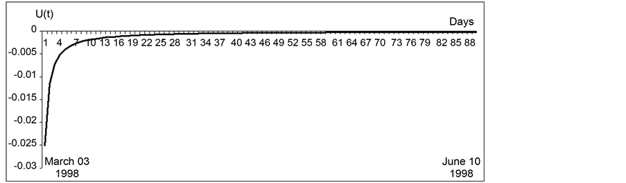
Figure 4. Interacting potential .
.

Figure 5. Simulated option price P (continuous line), Black-Scholes model price B-S (dashed line) and interacting Black-Scholes model price CPV (dotted line) for the e-mini S&P 500 contract from 12/03/1998 to 10/06/1998.
 (a)
(a) (b)
(b) (c)
(c) (d)
(d) (e)
(e) (f)
(f)
Figure 6. (a) (b) (c) (d) (e) (f): Simulated option price P (continuous line), Black-Scholes model price B-S (dashed line) and interacting Black-Scholes model price CPV (dotted line) for e-mini S&P 500 contracts in Table 1.
hence arbitrage processes form part of the normal operation of the stock exchange, and logically mispricing is always going to exist. If this mispricing could be calibrated using the potential of the interacting Black-Scholes, even in a small part, it is expected that those results are always going to outperform the traditional Black-Scholes formulation. In this context, this model and its calibration procedure could be used very easily to simulate in a more exact fashion option pricing of any underlying asset.
Future research could be directed to capture different potential patterns for different underlying assets and different market situations. Even in this case, the potential is short-lived and circumstantial, for example in the case of bubbles, rebounds, crises or critical information (for example, when Bernanke talked!), it is possible to use this methodology to capture the potential of the contract in a similar situation and to simulate the new contract. Alternatively, if the situation is normal and no special conditions are foreseen, a good practice would be to use the immediately preceding contract in order to calibrate the potential and therefore the quantum model; considering the reasons given above, in almost all the cases, it is expected that this model will defeat the traditional Black-Scholes model.
Cite this paper
Contreras, M., Pellicer, R., Santiagos, D. and Villena, M. (2016) Calibration and Simulation of Arbitrage Effects in a Non-Equilibrium Quantum Black-Scholes Model by Using Semi- Classical Methods. Journal of Mathematical Finance, 6, 541-561. http://dx.doi.org/10.4236/jmf.2016.64042
References
- 1. Black, F. and Scholes, M. (1973) The Pricing of Options and Corporate Liabilities. Journal of Political Economy, 81, 637-654.
http://dx.doi.org/10.1086/260062 - 2. Merton, R.C. (1973) Theory of Rational Option Pricing. Bell Journal of Economics and Management Science, 4, 141-183.
http://dx.doi.org/10.2307/3003143 - 3. Bjork, T. (1998) Arbitrage Theory in Continuous Time. Oxford University Press, Oxford.
http://dx.doi.org/10.1093/0198775180.001.0001 - 4. Duffie, D. (1996) Dynamic Asset Pricing Theory. 2nd Edition, Princeton University Press, Princeton.
- 5. Hull, J.C. (1997) Options, Futures, and Other Derivatives. Englewood Cliffs, Prentice-Hall.
- 6. Wilmott, P. (1998) Derivatives: The Theory and Practice of Financial Engineering. Wiley, Hoboken.
- 7. Contreras, M., Montalva, R., Pellicer, R. and Villena, M. (2010) Dynamic Option Pricing with Endogenous Stochastic Arbitrage. Physica A: Statistical Mechanics and Its Applications, 38, 3552-3564.
http://dx.doi.org/10.1016/j.physa.2010.04.019 - 8. Contreras, M., Pellicer, R., Ruiz, A. and Villena, M. (2010) A Quantum Model of Option Pricing: When Black-Scholes Meets Schrodinger and Its Semi-Classical Limit. Physica A: Statistical Mechanics and Its Applications, 389, 5447-5459.
http://dx.doi.org/10.1016/j.physa.2010.08.018 - 9. Otto, M. (2000) Stochastic Relaxational Dynamics Applied to Finance: Towards Non-Equilibrium Option Pricing Theory. The European Physical Journal B, 14, 383-394.
http://dx.doi.org/10.1007/s100510050143 - 10. Panayides, S. (2006) Arbitrage Opportunities and Their Implications to Derivative Hedging. Physica A: Statistical Mechanics and Its Applications, 361, 289-296.
http://dx.doi.org/10.1016/j.physa.2005.06.077 - 11. Fedotov, S. and Panayides, S. (2005) Stochastic Arbitrage Return and Its Implication for Option Pricing. Physica A: Statistical Mechanics and Its Applications, 345, 207-217.
http://dx.doi.org/10.1016/S0378-4371(04)00989-6 - 12. Ilinski, K. (1999) How to Account for the Virtual Arbitrage in the Standard Derivative Pricing. arXiv:cond-mat/9902047v1.
- 13. Ilinski, K. and Stepanenko, A. (1999) Derivative Pricing with Virtual Arbitrage. arXiv:cond-mat/9902046v1.
- 14. Ilinski, K. (2001) Physics of Finance: Gauge Modelling in Non-Equilibrium Pricing, Wiley, Hoboken.
- 15. Segal, W. and Segal, I.E. (1998) The Black-Scholes Pricing Formula in the Quantum Context. Proceedings of the National Academy of Sciences of the United States of America, 95, 4072-4075.
http://dx.doi.org/10.1073/pnas.95.7.4072 - 16. Haven, E. (2003) A Black-Scholes Schrodinger Option Price: “Bit” versus “Qubit”. Physica A: Statistical Mechanics and Its Applications, 324, 201-206.
http://dx.doi.org/10.1016/S0378-4371(02)01846-0 - 17. Haven, E. (2002) A Discussion on Embedding the Black-Scholes Option Price Model in a Quantum Physics Setting. Physica A: Statistical Mechanics and Its Applications, 304, 507-524.
http://dx.doi.org/10.1016/S0378-4371(01)00568-4 - 18. Baaquie, B. (2004) Quantum Finance. Cambridge University Press, Cambridge.
http://dx.doi.org/10.1017/CBO9780511617577 - 19. Schaeffer, R. (1978) Semi-Classical Approximation for Heavy Ions. In: McVoy, K.W. and Friedman, W.A., Eds., Theoretical Methods in Medium Energy and Heavy Ion Physics, Nato Advanced Studies Institute Series B, Springer, Berlin, 189-234.
http://dx.doi.org/10.1007/978-1-4613-2877-3_2 - 20. Gibbons, G.W. and Hawking, S. (1977) Action Integrals and Partition Functions in Quantum Gravity. Physical Review D, 15, 2752-2756.
http://dx.doi.org/10.1103/PhysRevD.15.2752 - 21. Keshavamurhy, S. (1994) Semi-Classical Methods in Chemical Reaction Dynamics. PhD Thesis, Chemistry Department University of California, Auckland.
- 22. Riva, V. (2006) Semi-Classical Methods in 2D QFT: Spectra and Finite Size Effects. PhD Thesis, Modern Physics Letters A, 21, 2099-2116.
http://dx.doi.org/10.1142/S0217732306021621 - 23. Chaichian, M. and Demichev, A. (2001) Path Integrals in Physics. Vol. I, Institute of Physics (IOP) Publishing, Bristol.
- 24. Baaquie, B.E. (1997) A Path Integral to Option Price with Stochastic Volatility: Some Exact Results. Journal de Physique, 7, 1733-1753.
- 25. Linetsky, V. (1998) The Path Integral Approach to Financial Modelling and Option Pricing. omputational Economics, 11, 129-163.
- 26. Bennati, E., Rosa-Clot, M. and Taddei, S. (1999) A Path Integral Approach to Derivative Security Pricing: I. Formalism and Analytical Results. International Journal of Theoretical and Applied Finance, 2, 381-407.
http://dx.doi.org/10.1142/S0219024999000200 - 27. Rosa-Clot, M. and Taddei, S. (2002) A Path Integral Approach to Derivative Security Pricing: II. Numerical Methods. International Journal of Theoretical and Applied Finance, 5, 123-146.
http://dx.doi.org/10.1142/S0219024902001377 - 28. Lemmens, D., Wouters, M. and Tempere, J. (2008) A Path Integral Approach to Closed-Form Option Pricing Formulas with Applications to Stochastic Volatility and Interest Rate Models. Physical Review E, 78, Article ID: 016101. arXiv:0806.0932v1
http://dx.doi.org/10.1103/PhysRevE.78.016101 - 29. Devreese, J.P.A., Lemmens, D. and Tempere, J. (2010) Path Integral Approach to Asian Options in the Black-Scholes Model. Physica A: Statistical Mechanics and Its Applications, 389, 780-788. arXiv:0906.4456v3
http://dx.doi.org/10.1016/j.physa.2009.10.020 - 30. Dash, J.W. (2016) Quantitative Finance and Risk Management: A Physicist’s Approach. 2nd Edition World Scientific Publishing Company, Singapore.
http://dx.doi.org/10.1142/9003 - 31. Kleinert, H. (2006) Path Integrals in Quantum Mechanics, Statistic, Polymer Physics, and Financial Markets. 4th Edition, World Scientific Publishing Company, Singapore.
http://dx.doi.org/10.1142/6223 - 32. Lo, A.W. and MacKinlay, A.C. (1999) A Non-Random Walk Down Wall Street. Princeton University Press.