Received 8 October 2015; accepted 27 November 2015; published 30 November 2015

ABSTRACT

We study the default risk in incomplete information. That means we model the value of a firm by a Lévy process which is the sum of a Brownian motion with drift and a compound Poisson process. This Lévy process cannot be completely observed, and another process represents the available information on the firm. We obtain a stochastic Volterra equation satisfied by the conditional density of the default time given the available information. The uniqueness of solution of this equation is proved. Numerical examples of (conditional) density are also given.

Keywords:

Conditional Density, Default Time, Lévy Processes, Filtering Theory, Stochastic Voltera Equations

1. Introduction

Here we consider a jump-diffusion process X which models the value of a firm. This is a Lévy process. Details on this class of processes can be found in [1] and [2] . Their use in financial modeling is well developed in [3] . We study the first passage time of process X at level modeling the default time. We investigate the behavior of the default time under incomplete observation of assets. In the literature, there exists some papers in relation to this topic. Duffie and Lando [4] suppose that bond investors cannot observe the issuer’s assets directly; instead, they only receive periodic and imperfect reports. For a setting in which the assets of the firm are geometric Brownian motion until informed equity holders optimally liquidate, they derive the conditional distribution of the assets, and give the available information. In a similar model, but with complete information, Kou and Wang [5] study the first passage time of a jump-diffusion process whose jump sizes follow a double exponential distribution. They obtain explicit solutions of the Laplace transform of the distribution of the first passage time. Laplace transform of the joint distribution of jump-diffusion and its running maximum, , is too obtained. To finish, they give numerical examples. Bernyk et al. [6] , for their part, consider stable Lévy process X of index with non negative jumps and its running maximum. They characterize the density function of as the unique solution of a weakly singular Volterra integral equation of the first kind. This leads to an explicit representation of the density of the first passage time. To unify the noisy information in Duffie and Lando [4] , X. Guo, R. A. Jarrow and Y. Zang [7] define a filtration which models incomplete information. By simple examples, they give the importance of this notion. Similarly to Kou and Wang, without specifying the jumps size law, Dorobantu [8] provides the intensity function of the default time. That is very important for investors, but the information brought by this intensity is low. Furthermore, Roynette et al. [9] prove that the Laplace transform of the random triplet (first passage time, overshoot, undershoot) satisfies an integral equation. After normalization of the first passage time, they show under some convenient assumptions that the random triplet converges in distribution as level x goes to. Gapeev and Jeanblanc [10] study a model of a financial market in which the dividend rates of two risky asset’s initial values change when certain unobservable external events occur. The asset price dynamics are described by a geometric Brownian motion, with random drift rates switching at independent exponential random times. These random times are independent of the constantly correlated driving Brownian motion. They obtain closed expressions for rational values of European contingent claims given the available information. Moreover, estimates of the switching times and their conditional probability density are provided. Coutin and Dorobantu [11] prove that the default time law has a density (defective when) with respect to the Lebesgue measure in case of a stationary independent increment process built on a pair (compound Poisson process, Brownian motion).

We extend this approach studying the conditional law of the first passage time of Lévy process at level x given a partial information. We solve this problem using filtering theory inspired by Zakai [12] , Pardoux [13] , Coutin [14] , Bain and Crisan [15] , based on the so called “reference probability measure” method. The paper is organized as follows: Section 2 sets the model; Section 3 gives the results on the existence of the conditional density given the observed filtration and on the integro-differential equation satisfied by this conditional density; Section 4 gives the proofs of the results. To finish, we conclude and give some auxiliary results in Appendix.

2. Model and Motivations

This section defines the basic space in which we work and announces what we will do. Subsection 2.1 gives the model of the firm value and defines the default time. Subsection 2.2 recalls some important results in the complete information case. Subsection 2.3 defines the signal and observation process and the model for available information. Basically, it introduces the notion of filtering theory. Subsection 2.4 gives our motivation.

2.1. Construction of the Model

Let be a filtered probability space satisfying the usual conditions on which we define a

standard Brownian motion W, a sequence of independent and identically distributed random variables

with distribution function, a Poisson process N with intensity and a stochastic process Q. We assume that all these elements are independent, is a Brownian motion and is a compound

Poisson process with intensity ν under defined for any Borel set A by. On this

probability space, we define a process X as follows:

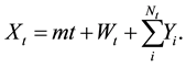(1)

X models a firm value and the default is modeled by the first passage time of X at a level. Hence the default time is defined as

. (2)

We suppose that X is not perfectly observable and that observation is modeled by process Q.

2.2. Some Results When X Is Perfectly Observed

Let be a Brownian motion with drift mÎR (). For, we let

By (5.12) page 197 of [16] , has the following law on:

(3)

where

The function is on, and all its derivatives admit 0 as right limit at 0 and therefore belongs

to. For, Roynette et al. [9] consider as a firm value the process and

as a default time the random variable They let namely overshoot and

namely undershoot. They prove that the Laplace transform of satisfies an integral equation. After a suitable renormalization of that we can note here, they show that converges in distribution as x goes to. Overall they have obtained an asymptotic behavior of the defaut time, the overshoot and the undershoot.

For a general Lévy process, Doney and Kiprianou [17] give the law of the quintuplet

where and.

Coutin and Dorobantu [11] consider (1) and (2) and show that admits a density with respect to the Lebesgue measure. They give the following closed expression of this density

(4)

where is the sequence of the jump times of the process N.

2.3. The Incomplete Information

Our work is inspired and is in the same spirit as D. Dorobantu [8] . In her thesis, Dorobantu assumes that investors wishing to detain a part of the firm do not have complete information. They don’t observe perfectly the process value X of the firm but a noisy value. She defined a process Q independent of and satisfying the following evolution equation

with h a Borel and bounded function and B a standard Brownian motion.

Definition 1. The process X is called the signal. The process Q is called the observation and is perfectly observed by investors.

This leads us to a filtering model and we introduce the filtering framework inspired of Zakai [12] , Coutin [14] or Pardoux [13] .

Since the function h is bounded, the Novikov condition, is satisfied and we

define the following exponential martingale for the filtration by

For a fixed maturity, the process is a uniformly integrable -martingale.

Definition 2. For fixed, let us define a probability measure on by

We also note that the law of X, so the one of, under is the same as under. Note that investors have additional information on the firm which is modeled at time t by

Then all the available information is represented by the filtration

where the s-algebra is generated by the observation of the process Q up to time t.

2.4. Motivations

D. Dorobantu [8] obtains the -intensity of the default, namely the -predictable process, such that

is a -martingale. With this result, using their available information, the investors can predict the default time. More precisely, given that default did not occur at time t, the probability that it occurs at time is

approximated by. But the information brought by the knowledge of is low. This motivates us to

show that the conditional law of default time given admits a density with respect to Lebesgue measure and to give its dynamic evolution.

This section presents our basic model of a firm with incomplete information about its assets. More generally, we treat a continuous time setting, staying with the work of D. Dorobantu [8] in her thesis second part. Next section gives our main results.

3. The Results

3.1. Existence of the Conditional Density

We recall that is the default time of a firm and is the available information of investors at time t. In this subsection, we prove that conditionally on the s-algebra, admits a density with respect to the Lebesgue measure.

Proposition 1. For all, on the set, the conditional law of has the following form

(5)

where

And

Remark 1 Referring to [9] , for all, the passage time is finite almost surely if and only if.

3.2. Mixed Filtering-Integro-Differential Equation for Conditional Density

In this subsection, we give our main results. Indeed, we first show that the conditional law of the hitting time

given the filtration satisfies a stochastic integro-differential equation. Afterwards, we give a uniqueness

result. This type of equation is the same as the one studied in [18] with the only difference that here, we have more general Voltera random coefficients.

Theorem 1. Let be a real number. For any, on the set, the conditional density of given satisfies the stochastic integro-differential equation:

(6)

where

and G is defined in Proposition 1.

Proposition 2. If Equation (6) admits a solution, this one is unique.

3.3. Some Technical Results

Here, we give some technical and auxiliary results which are useful to prove Theorem 1 and Proposition 2.

Proposition 3. For any bounded function such that is -measurable,

(7)

By this proposition, we establish two corollaries which give a representation more accessible of the processes

and: we apply Proposition 3 respectively to the functions and the second expressions being consequence of the fact that on the event

τ_x = u + (q is the shift operator) and

Corollary 1. For all we have

1) (8)

and equivalently

2) (9)

Corollary 2. For

1) (10)

and equivalently

2) (11)

Proposition 4. For any we have on the set

(12)

Remark 2. Equation (12) of Proposition 4 can be rewriten as:

Where

This equation is similar to the non normalized conditional distribution Equation (3.43) in A. Bain and D. Crisan [15] , called Zakai equation.

In the same way, Equation (6) which is derived from (12) is similar to the normalized conditional distribution Equation (3.57) in A. Bain and D. Crisan [15] , called Kushner-Stratonovich equation.

3.4. Numerical Examples

We simulate the density of the first passage time respectively in complete information and in incomplete information. We suppose that the jump size follows a double exponential distribution, i.e, the common density of Y

is given by where are constants, and.

Here, and. The difference between the figures is on one hand due to the

information and on another hand to the values taken by the parameters m and.

These four first figures (Figue 1 and Figure 2) represent the densities of the first passage time for a jump

diffusion process (case of complete information). The variable and Monte Carlo results are based on 5000 simulation runs.

Figure 3, Figure 4 and Figure 6 are those of the conditional density (case of incomplete information), for fixed and the variable r is such that. Part II of A. Bain and D. Crisan [15] , namely Numerical Algorithms, where the authors give some tools to solve the filtering problem is really useful. The class of the numerical method used is the particle method for continuous time framework.Here, the Monte Carlo results are based on 120 simulation runs.

We observe that the maximum reached is greater if the drift m is positive, meaning the positive level x is more probably reached in a shorter time.

In incomplete information, the distance between the curve and axis is greater than in complete information case, this would mean that in case of incomplete information, the level x is more difficult to be reached in a short time.

The choice of the small value of serves to compare the results with the limiting Brownian motion case (). In complete information case, the formulae for the first passage times of Brownian motion can be found in [16] .

A large value of implies a lot of jumps, a large computing time and less regular curve.

In these last four figures (Figure 5 and Figure 6), the maximum reached is greater if the drift m is negative, meaning the positive level x is more probably reached in a shorter time. This is due to the very small value of.

4. Proofs

Proposition 1

Proof. First note that, since X is a -Markov process and, we have

The fact that is a -stopping time justifies the last equality.

Secondly, for any the Markov property of the process X and the fact that on the set, ensure

The -conditional law of has the density (possibly defective), thus

By hypothesis, we have It follows from Lemma 3 of Appendix that

Then, we have for any

Now, we show the equality almost surely for all Let and be the processes defined by

These processes are increasing, then they are sub-martingales with respect to the filtration Note that and are too continuous. Using Revuz-Yor Theorem 2.9 p. 61 [19] , they have same càd-làg modification for all b, meaning that

We conclude that, almost surely, for all

Taking, letting n going to infinity and using monotone Lebesgue Theorem yield that,

□

Proposition 2

Proof. Let and be two solutions of Equation (6) and. It follows that

(13)

where

(14)

We recall the expression

and remark that. Then

Markov property implies

We use Lemma 4 with and and it follows that

and Lemma 7 (22) with the pair gets

.

All computations are done on the set. We observe too is a positive

submartingale. Then for all, we obtain by Lemma 7 (22) with the pair, Doob’s inequality and

.

Thanks to Jensen inequality and Lemma 8 with and, it follows that

Concerning the numerator, Since Novikov condition

is satisfied then is a locally square integrable -martingale. Once again Doob’s inequality gets

So finally

(15)

Let and. On the set,. Moreover (15) proves that so.

It follows using (13) that

Taking, we obtain

(16)

Then

.

By Gronwall’s lemma, we deduce that is the unique solution of (16) on the set, so

Uniqueness of solution of (6) is a consequence of. □

Proposition 3

Proof. Let be a process where the set of processes is defined in Lemma 5 and a time t. Lemma 7 applied to which belongs to implies

Conditioning by under the time integral, it follows that

Conversely compute the expectation of the product of by right hand of (7):

.

Since is dense in

Finally we could replace by its conditional expectation since □

Proposition 4

Proof. Applying Lemma 4, it follows that

(17)

But, since the condition is not necessarily satisfied, we are not able to prove

that is a semi martingale (e.g. see Protter’s Theorem 65 Chapter 4 [20] ). This leads us to

consider for the expression instead of at denominator of

(17). But Lemma 7 of Appendix ensures that

We apply Ito formula to the ratio of processes. For this end, we let two processes

satisfying the stochastic equations respectively (9) and (11):

The Itô’s formula applied to from 0 to t gives us

We achieve the proof letting using the monotonous Lebesgue theorem since increases to when. □

Theorem 1

Proof. Let us now find a mixed filtering-integro-differential equation satisfied by the conditional probability density process defined from the representation

(18)

We fix a and t such that. Let be, recalling the -Markov property of X at point u and the fact that justify

By definition of G, we have

Then

By Tonelli Theorem,

Similarly

In Equation (12) of Proposition 4,

are respectively replaced by

By hypothesis, we have.

For, Lemma 8 of Appendix ensures that

The numerators being bounded by, we can apply stochastic Fubini’s theorem to Equation (12) Pro-

position 4, which can be written again as

To express this result with conditional expectation instead of conditional expectation, each fraction

under the integral is multiplied and divided by the same term To manage the indicator func-

tion, we use the filtration since is a -stopping time.

Therefore, using (20) in Lemma 4, on the set we obtain

which finishes the proof. □

5. Conclusion

This paper extends the study of the first passage time for a Lévy process in [5] from complete to incomplete information and D. Dorobantu’s work in [8] from intensity to conditional density. Here, we are proving the existence of the density of law given an information set, giving a stochastic differential integral equation satisfied by it and some numerical examples. All this gives us a behavior of the default time. In future works, we will be interested by the same studies in discrete time, in another kind of information set or under another process modeling the firm value.

Acknowledgements

We thank my PhD advisor Laure Coutin for her help and pointing out error. We thank too Monique Pontier for her careful reading. We thank the Editor and the referee for their comments. This work is supported by A.N.R. Masterie. This support is greatly appreciated.

Cite this paper

WalyNgom,11, (2015) Conditional Law of the Hitting Time for a Lévy Process in Incomplete Observation. Journal of Mathematical Finance,05,505-524. doi: 10.4236/jmf.2015.55041

References

Appendix

Lemma 1. Let be and real numbers and G a Gaussian random variable with mean zero and variance one, then

Proof. Indeed using the law of G, we have

Since then

By change of variable, it follows that

□

Lemma 2. If is the sequence of jump time of the process N, then

Proof. We have

where is an exponential random variable with parameter and independent of which follows a Gamma law with parameters n and. Therefore

□

Lemma 3. There exists some constants and C such that

(19)

Proof. The function f defined in (4) satisfies

Using the fact that if then, we have

Replacing by its expression, we obtain

Let. We apply this bound to:

Remark that conditionally to process N and the, the law of the random variable is a

Gaussian law with mean and variance

Applying Lemma 1 we get the conditional expectation

Using the fact that we obtain since

The proof is completed with Lemma 2. □

The next lemma is inspired of Jeanblanc and Rutkovski [21] and Dorobantu [8] .

Lemma 4. For all for all a and b such that for all

(20)

For instance with we get

Proof. Assume that there exists such that Then for all It follows that the density function of f, defined in (4), is the zero function on. This means that,

Then, implies that

Thus But we have and on the set

Therefore, for all t ≥ t₀ Hence, we obtain

what is not possible. Indeed,

That means for all In particular, for,

Thus for any t, t, and

On the set, any -measurable random variable coincides with some -measurable random variable (cf. Jeanblanc and Rutkovski [21] p. 18). Then for all, there exists a -measurable random variable Z such that

Taking the conditional expectation with respect to, we get

This implies that

Using Kallianpur-Striebel formula (see Pardoux [13] ) and we obtain

□

The following is in [14] .

Lemma 5. The family of adapted processes

is total in the set of processes taking their values in

Let us denote by (resp. and) the completed, right continuous filtration generated by W, (resp. N or X)

Lemma 6. Let be an -progressively measurable process such that for all, we have

Then

(21)

Proof. As in Lemma 5, the family of processes

is total in the set of processes taking their values in where is the compensated Poisson random measure on and is a Borel set.

Therefore, since by Itô’s formula, we have

The equality is obtained from the fact that under, by independence. □

Lemma 7. Let be a process such that for any t . Let and, then

and

(22)

For instance

Proof. Let be and let us define the process K

The integration by parts Itô formula applied to the product between 0 and T yields

and remark that

Since X and Q are independent under, we use Lemma 6 and it follows

(23)

Similarly, using first Itô’s formula on product of processes

and the independence between X and Q under yields

. (24)

Equations (23) and (24) imply that

Now let be and apply the above equality to:

so

which concludes the proof. □

Lemma 8. For all, , almost surely and

Proof. The process is a positive (upper ) martingale, which converges to the non null random variable (see Lemma 4) then it never vanishes.

From Corollary 2 (i), the process is a martingale with decom-

position

Let using Itô’s formula for between 0 and and

taking the expectation we derive

Using Gronwall’s Lemma

The proof of Lemma 8 is achieved by letting n going to infinity. □

References

- 1. Bertoin, J. (1998) Lévy Processes. Vol. 121, Cambridge University Press, Cambridge.
- 2. Sato, K. (1999) Lévy Processes and Infinitely Divisible Distribution. Vol. 68 of Cambridge Studies in Advanced Mathematics, Cambridge University Press, Cambridge, Translated from the 1990 Japanese Original, Revised by the Author, 1999.
- 3. Cont, R. and Tankov, P. (2004) Financial Modeling with Jump Processes. Chapman & Hall/CRC, Boca Raton, London, New York.
- 4. Duffie, D. and Lando, D. (2001) Term Structure of Credit Spreads with Incomplete Accounting Information. Econometrica, 69, 633-664.
http://dx.doi.org/10.1111/1468-0262.00208 - 5. Kou, S.G. and Wang, H. (2003) First Passage Time of a Jump Diffusion Process. Advances in Applied Probability, 35, 504-531.
http://dx.doi.org/10.1239/aap/1051201658 - 6. Bernyk, V., Dalang, R.C. and Peskir, G. (2008) The Law of the Supremum of a Stable Lévy Process with No Negative Jumps. The Annals of Probability, 36, 1777-1789.
http://dx.doi.org/10.1214/07-AOP376 - 7. Guo, X., Jarrow, R. and Zeng, Y. (2009) Credit Model with Incomplete Information (Earlier Version Information Reduction in Credit Risk Models). Mathematics of Operations Research, 34, 320-332.
http://dx.doi.org/10.1287/moor.1080.0361 - 8. Dorobantu, D. (2007) Modélisation de risque de défaut en enterprise. Thèse de l’Université de Toulouse 3.
- 9. Roynette, B., Vallois, P. and Volpi, A. (2008) Asymptotic Behavior of the Hitting Time, Overshoot and Undershoot for Some Lévy Processes. ESAIM: PS, 12, 58-93.
- 10. Gapeev, P.V. and Jeanblanc, M. (2010) Pricing and Filtering in Two-Dimensional Dividend Switching Model. International Journal of Theoretical and Applied Finance, 13, 1001-1017. http://dx.doi.org/10.1142/S021902491000608X
- 11. Coutin, L. and Dorobantu, D. (2011) First Passage Time Law for Some Lévy Process with Compound Poisson: Existence of a Density. Bernoulli, 17, 1127-1135. http://dx.doi.org/10.3150/10-BEJ323
- 12. Zakai, M. (1969) On the Optimal Filtering Diffusion Process. Zeitschrift für Wahrscheinlichkeitstheorie und Verwandte Gebiete, 11, 230-249.
http://dx.doi.org/10.1007/BF00536382 - 13. Pardoux, E. (1991) Filtrage non linéaire et équations aux dérivées partielles stochastiques associées. Ecole d’Eté de Probabilités de Saint-Flour-1989, Lecture Notes in Mathematics 1464, Springer-Verlag, Heidelberg, New York.
- 14. Coutin, L. (1996) Filtrage d’un système càd-làg: Application du calcul des variations stochastiques à l'existence d'une densité. Stochastics and Stochastics Reports, 58, 209-243.
http://dx.doi.org/10.1080/17442509608834075 - 15. Bain, A. and Crisan, D. (2009) Fundamentals of Stochastic Filtering. Springer-Verlag, New York.
http://dx.doi.org/10.1007/978-0-387-76896-0 - 16. Karatzas, I. and Shreve, S.E. (1991) Brownian Motion and Stochastic Calculus. Second Edition, Springer-Verlag, New York.
- 17. Doney, R.A. and Kiprianou, A. (2005) Overshoot and Undershoot of Lévy Process. The Annals of Applied Probability, 16, 91-106.
http://dx.doi.org/10.1214/105051605000000647 - 18. Protter, P. (1985) Volterra equations driven by semi martingale. Annals of Probability, 13, 518-530.
http://dx.doi.org/10.1214/aop/1176993006 - 19. Revuz, D. and Yor, M. (1999) Continuous Martingales and Brownian Motion. Third Edition, Springer-Verlag, Berlin, Heldelberg, New York.
http://dx.doi.org/10.1007/978-3-662-06400-9 - 20. Protter, P. (2003) Stochastic Integration and Differential Equation. Second Edition, Springer, Berlin.
- 21. Jeanblanc, M. and Rutkowski, M. (2000) Modeling of Default Risk: Mathematical Tools, Mathematical Finance; Theory and Practice. Modern Mathematics Series, High Education Press.
Appendix
Lemma 1. Let be  and
and  real numbers and G a Gaussian random variable with mean zero and variance one, then