Journal of Mathematical Finance
Vol. 3 No. 3A (2013) , Article ID: 38565 , 9 pages DOI:10.4236/jmf.2013.33A006
Can Banks Circumvent Minimum Capital Requirements? The Case of Mortgage Portfolio under Basel II
Department of Supervision, Regulation, and Credit, Federal Reserve Bank of Philadelphia, Philadelphia, USA
Email: Julapa.Jagtiani@phil.frb.org
Copyright © 2013 Christopher Henderson, Julapa Jagtiani. This is an open access article distributed under the Creative Commons Attribution License, which permits unrestricted use, distribution, and reproduction in any medium, provided the original work is properly cited.
Received August 22, 2013; revised September 25, 2013; accepted October 11, 2013
Keywords: Basel II; Bank Capital; Bank Regulation; Mortgage Default; Retail Credit Risk
ABSTRACT
The recent mortgage crisis has resulted in several bank failures. Under the current Basel I capital framework, banks are not required to hold a sufficient amount of capital to support the risk associated with their mortgage activities. The new Basel II capital rules are intended to be more risk based and would require the right amount of capital buffer to support bank risk. However, Basel II models could become too complex and too costly to implement, often resulting in a trade-off between complexity and model accuracy. Since the Basel II rules are meant to be principal based (rather than prescriptive), banks have the flexibility to build risk models that best fit their unique structure. We find that the variation of the model, particularly how mortgage portfolios are segmented, could have a significant impact on the default and loss estimated. This paper finds that the calculated Basel II capital varies considerably across the default prediction model and segmentation schemes, thus providing banks with an incentive to choose an approach that results in the least required capital for them. We find that a more granular segmentation model produces smaller required capital, regardless of the economic environment. Our results suggest that banks may have incentives to build risk models that meet the Basel II requirement and still yield the least amount of required capital.
1. Introduction
The recent U.S. mortgage crisis has caused upheaval in financial and payment systems around the globe. The dramatic growth in subprime mortgages, in conjunction with the decline in lending standards in the early and mid-2000s put the entire U.S. banking industry at great risk. A number of financial institutions have been closed, and those considered systemically important were rescued by the federal government during the financial crisis of 2007 and the ensuing recession. It has been evident that banks were not holding sufficient amounts of capital as a cushion to support their risky mortgage activities, causing them to become insolvent as the number of mortgage defaults increased as house prices declined and job losses mounted1.
The current Basel I capital requirement does not take into account the credit risk of mortgages; rather, it considers all mortgage assets to have a 50% risk weight regardless of the creditworthiness of the borrowers or the level of systemic risk in the economy. The objective of the Basel II framework is to enhance banks’ risk measurement and capital adequacy without being too prescriptive. The Basel II rule allows banks the flexibility to develop their own internal models that are appropriate to the organization’s risk profile and unique business model. While this is the strength of the Basel II framework, it is also one of the drawbacks. The flexibility allowed under the Basel II framework could result in banks choosing to adopt an internal model approach that yields the least amount of required capital. That is, variations of the modeling approaches could have a significant impact on the calculated required capital, holding fixed the risk that banks take, and, thus, could result in a level of required capital that is not correct and may be insufficient to cover unexpected losses especially during economic downturn conditions.
The next section presents a review of the literature related to the impacts of choices of credit risk models on bank capital. Section 3 provides a summary of the literature related to the importance of bank supervisory oversight to ensure adequate capitalization in the banking industry. The data are described in Section 4. Sections 5 presents the logistic default models that are used as segmentation criteria. Section 6 demonstrates the variation of required capital across the various segmentation approaches. Finally, Section 7 concludes our findings and discusses policy implications.
2. Literature Review
Given the novelty and complexity of the A-IRB approach of Basel II, and the limited knowledge of the importance of portfolio segmentation in measuring a bank’s risk exposure in retail lending activities, it is not surprising to see a sparse literature on this subject. References [2,3] provide an overview of issues in credit risk modeling for retail portfolios. Reference [4] focuses on the tail risk of mortgage lending. They argue that owing to the extreme skewness of returns from mortgage products, where loan losses are usually small but would rise sharply in the event of a severe financial crisis, Basel II capital calculation tends to understate tail risk in an extreme systemic crisis and, thus, could substantially underestimate the appropriate amount of prudential capital adequacy. Reference [5] find another potential reason for the Basel capital framework to provide inadequate capitalization focusing on subprime mortgages as the subprime defaults tend to be highly correlated.
A few studies have examined issues related to retail portfolio segmentation and the capital implications. In general, for products with a very large customer base such as mortgages, banks have the option to go with a very fine or a rough segmentation approach. Reference [6] utilizes auto lease financing data from European financial institutions in 2002 and finds that segmentation on the basis of scoring reduces the capital requirement by 30 basis points. This is consistent with the argument that banks could reduce their capital requirements for car loans through their choice of PD segmentation as well. Reference [7] uses auto loan data from 2000 to 2002 and finds similar results.
Reference [8] point out conceptually that banks have an incentive to estimate their PDs at a more granular level, because capital factors are concave in PD for a given LGD under the Basel II one-factor model, and because PDs are generally estimated at a more granular level than the LGD estimates. We demonstrate empirically in this paper that the bank’s choice of PD segmentation could reduce the required capital for mortgage portfolios.
Reference [9] examines the Basel II required capital for credit cards, using proprietary data from Capital One for credit card accounts originated in 1999 and 2000, with a performance period up to September 2004. They compare a simple segmentation approach (with only two factors: refreshed risk score and delinquency status) with a one-factor segmentation scheme. Their results suggest that the two-factor segmentation scheme produces lower required capital than the one-factor scheme. We perform a more in-depth analysis in this paper, focusing on mortgage—using data from 2000 to 2009 and exploring segmentation alternatives that contain up to 31 terminal nodes, including several additional important risk factors for segmentation criteria.
3. Bank Incentives to Circumvent Capital Requirements
Reference [10] details how banks prefer low-risk loans but pursue high portfolio risk in order to maximize their deposit insurance put option value. It is possible to characterize the incentive for banks to choose an internal model that yields the least amount of required capital using the put option value framework. Federal deposit insurance makes depositors willing to supply an unlimited amount of deposits at the riskless rate, regardless of the bank’s asset risk or leverage. We characterize the interaction between regulatory oversight and capital adequacy by modeling the expected return to bank equity holders by selecting feasible levels of portfolio risk and financial leverage as proxied by the deposit to capital ratio.
Following [10], risk-neutral bank shareholders seek to maximize their expected end-of-period wealth (W) by choosing positive deposit levels (D) and the loan portfolio’s riskiness (σp). Expected terminal wealth is given by
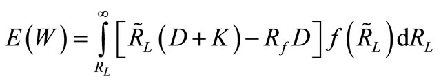 , where
 = one plus the riskless interest rate,
 = one plus the realized loan rate,
 =
= 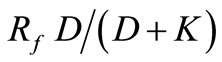 is the lowest loan return for which depositors can be fully repaid, and
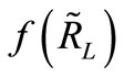 = the density function for
  (which depends on (σp)).
As a result, the option value, which is expressed per dollar of invested equity, can be rewritten in terms of a put option value (V):
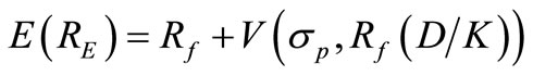 where
where  is the exercise price.
Reference [10] shows that additional leverage is obtained only from less asset risk but that endogenous bank practices could result in increases in both the bank’s option value and asset risk, ceteris paribus, resulting in an ambiguous impact on the option value (V). Based on this paper’s hypothesis that banks can systematically lower capital requirements by modeling more granular portfolio segments, we argue that the bank’s measure of portfolio risk using segmentation schemes outweighs any offsetting influence of endogenous bank practices, as it is the only way a bank can circumvent regulatory influence. Endogenous bank practices are observable to regulators. This implies that , where
  is the portfolio variance for the ith segment scheme and is less than the total loan portfolio variance for all i’s.
Unlike in [10], where the banks are free to choose individual loan risk, asset correlations, and portfolio composition, we argue that banks have incentives to choose the segmentation scheme that maximizes the put option value (V*). Imposing the regulatory constraint by introducing Basel II to affect permissible leverage, we model the constraint as a function of segmentation-driven portfolio variance such that ,
, . By imposing that the put option value is concave in
 , regulators constrain the bank’s maximum attainable option value (V*) by choosing
  that equates V* with the required regulatory capital levels. In this paper, we are concerned with a bank’s ability to identify and measure credit risk for estimation of required capital using their own internal models that are not independently validated and consistently monitored by banking regulators2. We argue later that regulatory oversight is critical to ensuring that banks do not exploit the benefit of reducing regulatory capital by investing in more granular segmentation systems.
4. The Data
Our primary source of data is the loan-level monthly mortgage data from the Lender Processing Services, Applied Analytics (LPS) database, which includes all mortgage loans from 9 out of 10 major servicers and which accounted for approximately 75 percent of all mortgage loans outstanding in the U.S. as of year-end 2009. We take a 5 percent random sample of observations and exclude those loans that were originated before 2000 or have missing FICO scores at origination. Our sample consists of approximately 2.46 million mortgage loans, originated during the period 2000-2008, a total of approximately 75.4 million monthly observations.
For the purpose of our analysis, we divide the monthly data for each loan into cohorts, with December 31 of each year being the observation date and the 12 months following being the outcome period. The LPS monthly data are divided into nine cohorts, with the cohort observation dates being December 31 of each year (2000- 2008), with the 12 months following each cohort date being the performance period for the cohort. For examplethe performance period for the December 31, 2000 cohort is the period January 1 to December 31, 2001. The first six cohorts are defined as pre-crisis cohorts, consisting of cohort observation dates December 31, 2000 to December 31, 2005—with the cohort observation period from January 1, 2001 to December 31, 2006. This includes mortgage loans originated between 2000 and the cohort date, where the default is defined based on the performance period (12 months following the cohort date). Similarly, the last three cohorts are defined as crisis cohorts, consisting of cohort observation dates December 31, 2006 to December 31, 2008—with the cohort observation period from January 1, 2007 to December 31, 2009.
The performance period data are used to define default within 12 months after the observation date. A loan is considered in default if it becomes at least 60 days past due during any part of the 12-month period following the cohort date. Once the default has been identified (based on monthly LPS data), the analysis includes only the year-end (cohort-level) data; this brings the number of observations down to 2.43 million for the pre-crisis period and 3.69 million for the crisis period. The LPS loanlevel data are then merged with the quarterly credit bureau data from the Equifax database for the same time period, using year-end data for the period 2000-2009. The Equifax data contain customer information, includeing all information about first mortgages, second mortgages, and all credit card loans. The primary purpose of merging these two data sets is to obtain additional information about the loans and the borrowers, which is not available from the LPS database—such as information about second liens for the same property (or “piggybacks”) and credit card utilization. Following the merging approach used in [11] we merge the LPS and Equifax data based on the following characteristics of first mortgage loans: open date, initial loan balance, and ZIP code. Unlike in [11] we exclude all first mortgage loans that are associated with customers who have more than one first mortgage. This is to ensure that we can match all the second mortgage loans of the same customer with the correct first mortgage loan and to ensure that the loans belong to the same property for the purpose of calculateing the combined loan-to-value (CLTV) ratio. The merging of our cohort level (year-end) LPS data with the Equifax data results in the final loan observations of 211,061 for the pre-crisis period and 329,854 for the crisis period.
Our economic data include (state-level) home-price index data from the Federal Housing Finance Agency (FHFA), formerly the Office of Federal Housing Enterprise Oversight (OFHEO), and the number of initial unemployment claim applications collected from the Haver Analytics database. The HPI is a weighted repeat-sales index based on mortgage transactions on single-family properties (purchased or securitized by Fannie Mae or Freddie Mac) and within the conforming amount limits.
Table 1 presents a summary description of the combined data set for the pre-crisis and crisis periods. The statistics presented for the pre-crisis period are calculated based on loans originated during the period 2000-2005 only. Data for the crisis period include loans that were originated prior to the crisis as well, that is, loans originnated during the period 2000-2008, with the default events occurring during the period 2007-2009. All statistics related to loan characteristics at origination include only loans that were originated during the period 2000-2005 (pre-crisis) and 2007-2009 (crisis). It is obvious from the summary statistics in Table 1 and the plot of vintage curves in Figure 1 that both lending standards and loan quality had deteriorated over the sample period, resulting in an increasing default rate from the pre-crisis to the crisis periods.
Pre-crisis data include loans originated in 2000-2005, with performance period 1/1/2001-12/31/2006. Crisis data include loans originated in 2000-2008, with performance period 1/1/2007-12/31/2009. Factors measured at originnation are calculated based on loans that were originated in 2000-2005 (Pre-Crisis) and 2007-2008 (Crisis).
5. Mortgage Default Model and Statistical Results
The logistic (mortgage) default models are then used in
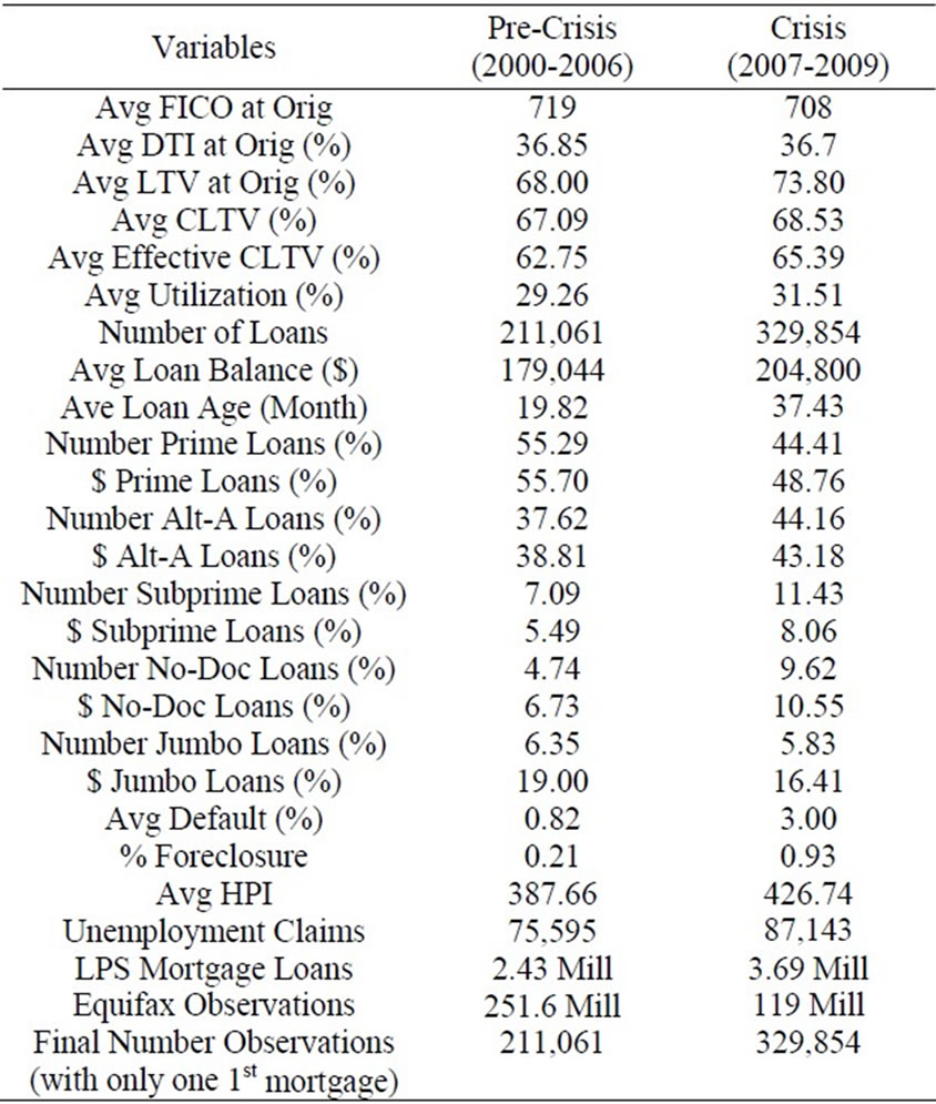
Table 1. Basic descriptive statistics.
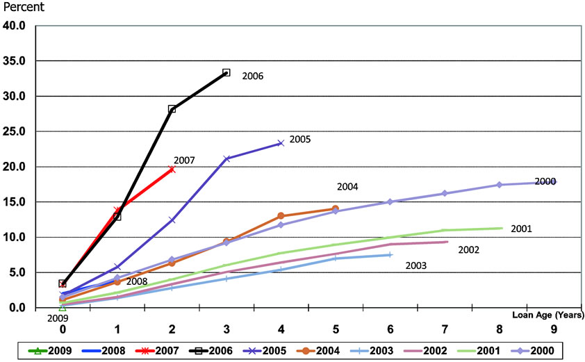
Figure 1. Vintage curve all mortgages, 2000-2009.
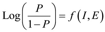
the next stage to build segments that are statistically meaningful. In the process of constructing meaningful segmentation schemes, we build five different (mortgage) default models with varying degrees of granularity— Model (1) is the least granular and Model (5) is the most granular. Logistic regressions are used to examine important factors that determine mortgage defaults, as defined in Equation (1) below.
 (1)
(1)
where P is the probability that the loan would default (default is defined as at least 60 days past due) within the next 12 months following the cohort date, while I and E are idiosyncratic and economic risk factors, respectively3. The variable P takes a value of 1 if the loan defaulted during the following 12-month outcome period, and zero otherwise.
The results of the logistic regression analysis, based on Equation (1), are reported in Table 2 for the crisis period4. Model (1) includes only product type (prime, alt-A, or subprime) and geographic region5. In Model (2), loan age as measured by months on book is included as well. Model (3) incorporates economic factors (home price index and unemployment) at the state level into the analysis; thus, there is no need to keep the geographic dummy variables that were included in Models (1) and (2). Model (4) includes five important credit risk factors: FICO score at origination (FICO), debt-to-income ratio
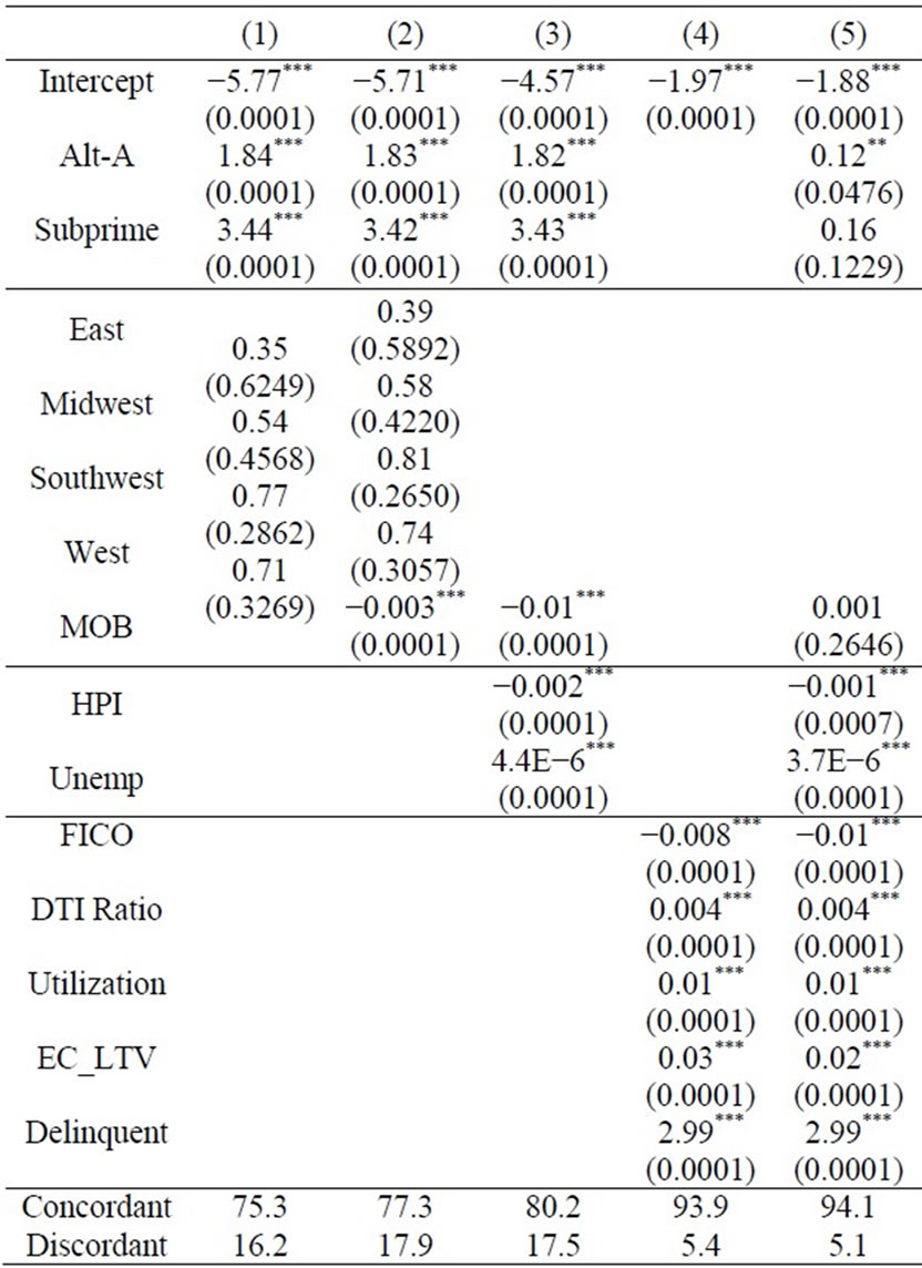
Table 2. Logistic analysis: Crisis period (2007-2009).
at origination (DTI), combined card utilization ratio (Utilization), effective combined loan-to-value ratio (EC_LTV), and spot delinquency, which is defined as 30+ days past due as of the cohort observation date (Delinquency)6. Following [11], the utilization ratio is used here as a measure of the borrower’s liquidity, where lower card utilization ratio is associated with better access to liquidity.
The results overall demonstrate the relationship between mortgage defaults and the various idiosyncratic risks associated with the loans, borrowers, product types, and economic factors. The borrower’s risk characteristics in Model (4) seem to be the most powerful of all idiosyncratic risk factors, as they fit the PD model the best (in terms of predictive ability of default) during the precrisis period, with 95.5 percent concordant. Adding the economic factors as in Model (5) does not improve the model’s predictive ability. One of the reasons may be that our credit risk factors have incorporated information related to economic conditions (particularly the home price index) through our EC_LTV variable7.
Results for the crisis period show that Model (5) performs slightly better than Model (4) —with 94.1 percent concordant compared with 93.9 percent. The economic factors do provide some additional information not captured by the credit risk factors during the financial crisis. The variable HPI is significant in Model (5) (at the 1 percent level) during the financial crisis period. This is consistent with the findings in [13] that the house price decline during the mortgage crisis eroded home equity, resulting in higher defaults not only among less creditworthy borrowers but also among prime borrowers8. The factors included in each of these models are then used for PD segmentation: five different segmentation schemes from Model (1) being least granular to Model (5) being the most granular. The first two models may be considered judgment-based segmentation models, since they leverage business expertise in devising the segmentation schemes, supported by judgment used in normal business practices. The last three models are considered more granular and are primarily statistics-based, using decision-tree methods to determine key risk drivers that differentiate risk within a retail portfolio.
We explore the various alternative segmentation schemes (with varying degrees of granularity) that meet these segmentation objectives and demonstrate that different qualified segmentation approaches could result in significantly different required capital and that banks may have incentives to choose a segmentation scheme that helps reduce their regulatory capital burden or promote capital avoidance.
The analysis reported in this table is based on Equation (1). Dependent variable is the probability of default (60+ dpd) in the next 12 months. Model (1) is the least granular model, including only product type and geographic factors. Model (2) includes months on book (MOB) as well. Model (3) includes economic variables, product type, and MOB. Model (4) includes idiosyncratic risk factors. Model (5) is the most granular, including all but regional factors, (regional impact is already incorporated into the analysis through HPI and unemployment). P-values are reported in parentheses. The ***, **, and * denote the 1%, 5%, and 10% significance, respectively.
6. Does the Required Capital Vary Across Segmentation Approaches?
The various Basel II risk parameters (PD, LGD, EAD) are calculated for each segment using the CHAID algorithm, and the required capital is calculated for the entire mortgage portfolio9. CHAID is also commonly used in the banking industry for the purpose of classifying data used in credit risk models. It involves formulating a set of rules that generate a split from a parent node to a child node based on the maximum similarity statistic within and between the nodes, to determine how records from the parent node are to be distributed across the child nodes. The CHAID tree diagram allows for multiple ways to split the observations into many categories (segments) based on categorical predictors within many classes10.
6.1. Probability of Default (PD)
The average PD for each node (segment) is calculated as the ratio of defaulted accounts to the total number of accounts in the node, where default is defined as being at least 60 days past due during the 12 months following the cohort date (observation date). Based on the PD of each node, we calculated average PDs for the entire mortgage portfolio using three different approaches: 1) simple average across nodes; 2) balance-weighted average PD, where the ratio of loan balance for each node to total loan balance for the portfolio is used as the weight; and 3) account-weighted average PD, where the ratio of the number of accounts for each node to the total number of accounts in the portfolio is used as the weight.
The Capital (K) in this table is calculated based on the Basel II formula for mortgages, where the asset correlation is 0.15. The LGDs used are based on three different assumptions for recovery cost (40%, 60%, and 80%).
The results are presented in Table 3. Average PDs vary greatly across the calculation method (simple average vs. balance weight vs. account weight) and vary across the segmentation approaches from Model (1) to Model (5). The account-weight PDs do not vary across models because default is calculated based on number of accounts. The simple average method tends to over-estimate the PD during good times, since there are a smaller number (or amount) of loans in bad segments, but could underestimate the PDs during bad times. The balance-weight method tends to produce the smallest estimated PDs regardless of model granularity or economic environment.
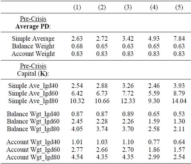
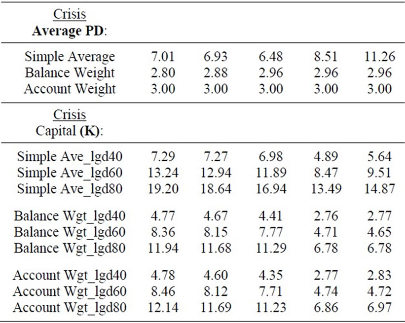
Table 3. Basel II Capital (K)—By Segmentation schemes and LGD assumption.
Our results suggest that a bank’s choice of PD estimation weighting method could also significantly affect the amount of required capital.
6.2. Loss given Default (LGD)
The parameter LGD is allowed to vary in our analysis due to the hypothetical nature of the portfolios. Under the Basel II framework, LGD is the bank’s empirically based best estimate of the economic loss, per dollar of exposure at default (EAD), that the bank would expect to incur if the exposures in the segment were to default within a one-year horizon during economic downturn conditions11.
In this study, we use the same segmentation schemes for both PD and LGD. The LGD is calculated based on foreclosed accounts in the PD segments, and it is equal to the ratio of the loss amount to the account balance prior to foreclosure. We provide several ranges for LGD based on industry practices to establish various sensitivities for LGD in order to test the robustness of the capital estimates for different loss severities that could be observed in actual bank portfolios over a range of economic conditions. That is, we estimate LGD from three different assumptions about the recovery cost (40, 60, and 80 percent). The loss amount is equal to the account balance minus the current value of the property (appraised value at origination adjusted by the HPI) plus the recovery cost. Following the Basel II final rules for mortgage LGD, the calculated LGD is floored at 10 percent and capped at 100 percent (at the loan level).
6.3. Basel II Capital (K), Risk-Weighted Assets (RWA), and Required Capital
K is calculated using the Basel II regulatory capital function, where the asset correlation (R) is equal to 0.15 as defined by the Basel II final rules for mortgages. The K is calculated for each segment based on the segment’s PD, LGD, and R, with three different recovery cost assumptions and is a key element in the calculation of required capital. The calculated Ks (for the entire mortgage portfolio) are reported in Table 3—top panel for precrisis and bottom panel for crisis—for the five different segmentation approaches (Model (1) to Model (5)) and across three different approaches for averaging across segments (simple average vs. balance-weighted average vs. account-weighted average). Again, the calculated K varies across the segmentation approaches and the methods of calculating average K. Using a simple average approach, the K value increases with the model granularity; thus, the least granular model produces less required capital. From the calculated K for each node, we also calculated the RWA for each segment (node), and it is equal to K*12.5*EAD, where the exposure at default (EAD) is the dollar amount of loan balance prior to foreclosure. The portfolio’s RWA is equal to the combined RWA across all segments, and the required tier I capital is equal to 8 percent of RWA, as reported in Table 4 for the five segmentation models—top panel for pre-crisis and bottom panel for crisis.
The dollar amount of required capital reported in this table is calculated based on the Basel II capital (K) for each node, the LGD for each node, and the EAD for each node (equal to loan balance). The $ amount of capital calculated for each of the nodes is then added together to derive the $ capital required for the mortgage portfolio. The node LGD is calculated based on three different recovery cost assumptions (40%, 60%, and 80%) and LGD
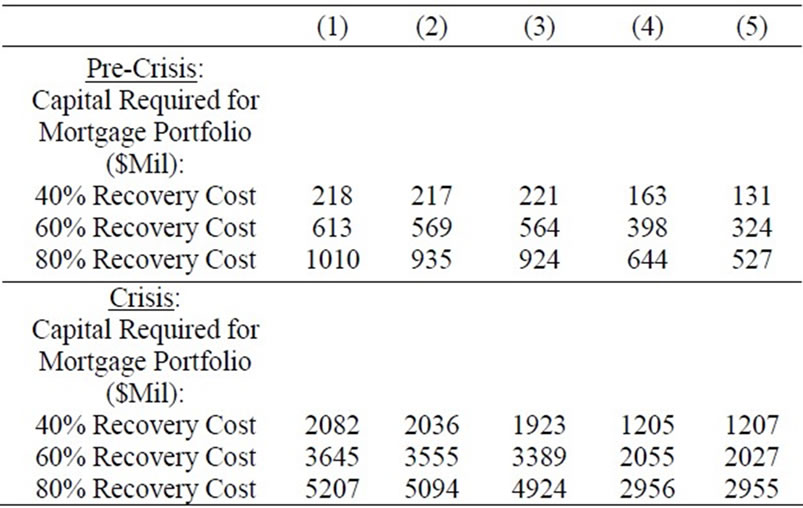
Table 4. Basel II Capital for Mortgage Portfolio by Segmentation Schemes and LGD Assumption.
is floored at 10% and capped at 100% (following the Basel II final rules).
The results reported in Table 4 demonstrate that required capital declines as the granularity of the segmentation scheme increases (consistent with the average K calculation using the balance-weighted method since it is EAD-weighted here)—moving from Model (1) to Model (5) would result in a capital reduction of 40 to 48 percent depending on the LGD assumptions. Note that the RWA here is calculated at the segment level and added across all segments. The RWA number could be significantly different if banks choose to calculate their portfolios’ RWA based on an average K for the portfolio (rather than segment), as the bank’s choice of calculation for the portfolio’s average K would directly impact the RWA and the required capital. Overall, our results indicate potential incentives for banks to choose a segmentation approach and RWA calculation method that help reduce the required capital for them.
7. Are More Granular Segmentation Schemes More Stable?
7.1. K-S and ROC Charts
In evaluating and comparing the quality of the various segmentation schemes, we plot the Kolmogorov-Smirnov (K-S) chart and the receiver-operator characteristics (ROC) chart (not shown but available upon request), for both the pre-crisis and post-crisis periods. The K-S plot shows that the K-S statistics range from 0.5701 in Model (1) to 0.8184 in Model (5), suggesting a better segmentation outcome for more granular models (in terms of homogeneity within segments and risk ranking across segments).
The ROC curve is a graphical representation of the trade-off between the false negative and the false positive. The larger the area under the curve, the better it is for the segmentation scheme in producing segments with homogeneous loans. The plots shows that Models (4) and (5), which include idiosyncratic credit risk factors, are superior to the less granular segmentation schemes in Model (1) to Model (3). Overall, the analysis suggests improved segmentation schemes with greater granularity.
7.2. Population Stability Index (PSI)
This is a measure of the stability of the segmentation over time, comparing the proportion of the population (mortgage loans) in each year that falls into each segment. We calculate PSI as indicated in Equation (2) below:
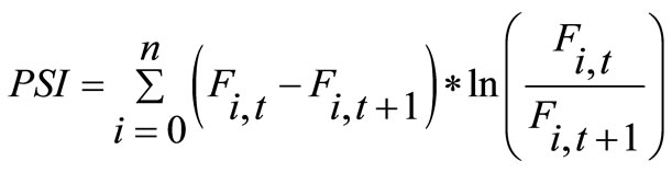 (2)
(2)
where Fi,t is the proportion of loans in Cohort (t) that falls in segment (node) i and Fi,t+1 is the proportion of loans in Cohort (t + 1) that falls in segment i.
A PSI index of 0.10 or less indicates no real population shift or a stable segmentation, and an index greater than 0.25 indicates a definite population shift and that the segmentation is not stable. An index between 0.10 and 0.25 suggests some shift in population.
Table 5 reports the PSI for both the pre-crisis and crisis periods. The results indicate that Models (3) and (2), in which PD segmentation schemes are based on economic factors, geographic indicators, and loan age only, are the least stable ones, during both the crisis and precrisis periods. The most granular segmentation schemes in Model (4) and Model (5) are not only more stable (with smaller PSI) but also produce a smaller estimated required capital for the bank (based on RWA calculated at the segment level, as shown in Table 4).
The PSI calculation is based on the proportion of loans in each cohort that falls into each node, using Equation (2). PSI < 0.10 indicates no real change from one cohort to the next. The ** denotes PSI between 0.10 and 0.25 (suggesting some shift), and *** denotes PSI > 0.25 (indicating a definite change in population from one cohort to the next).
8. Conclusions and Policy Implications
The recent mortgage crisis and the Great Recession that
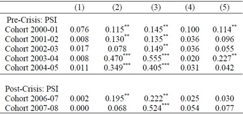
Table 5. Stability of the PD segmentation—Population Stability Index (PSI) by segmentation schemes.
followed resulted in several bank failures as the number of mortgage defaults increased as house prices plummeted. The current Basel I capital framework does not require banks to hold sufficient amounts of capital to support their mortgage activities, since all mortgages are treated as if they were equal in terms of riskiness, regardless of the borrower’s credit risk or whether they are noor low-documentation mortgages. The new Basel II capital rules and proposed Basel III rules are intended to correct this problem. However, Basel II models could become too complex and too costly to implement, resulting in a trade-off between complexity and model accuracy. More importantly, the variations in the models, particularly how mortgage portfolios are segmented, could potentially have a large impact on the default probabilities and estimated losses, thus significantly affecting the amount of capital that banks are required to hold.
Overall, we find that banks have the flexibility to choose an approach for their required capital calculation that meets the risk-based Basel II capital framework yet produces the least amount of capital thereby resulting in potential under-capitalization during economic downturn conditions. It is important that banks provide analytical support to regulators for important modeling assumptions to demonstrate that the segmentation system reflects risk drivers that are commonly found in the bank risk management process and that the segmentation system provides accurate, reliable, and consistent estimates of all the Basel II risk parameters (PD, LGD, and EAD). Furthermore, given banks’ ability to leverage their own internally developed risk parameters to calculate credit risk capital requirements, a formal periodic review (i.e. postqualification for Basel II or Pillar 2) would be necessary to ensure that the segmentation system is reviewed and updated appropriately to reflect a rapidly changing environment and economic impacts12.
Our results not only fill the gap in the literature regarding the impact of model segmentation, but they also serve as a benchmark modeling exercise using standard assumptions and analytical support for consistent and onsite examination to assess the implementation of the new Basel II risk-based capital requirement framework. It is important that banks choose the approach that is most appropriate for the risk profiles of their organizations in order to derive the most accurate risk measures and required capital for their retail portfolios.
9. Acknowledgements
The authors thank Larry White, Bill Lang, Paul Calem, Eli Brewer, Tim Opiela, Nicholas Kiefer, and participants at the FMA, WEA, SFA, and MFA conferences and the Interagency Risk Quantification Forum for their helpful comments and suggestions. Thanks also to Joanne Chow, Vidya Nayak, and Ali Cannoni for their dedicated research assistance. The paper received Best Paper Award at the 2011 Midwest Finance Association Conference. The opinions in this paper are the authors’ opinions and not necessarily those of the Federal Reserve Bank of Philadelphia or the Federal Reserve System.
REFERENCES
- W. Lang and J. Jagtiani, “The Mortgage and Financial Crises: The Role of Credit Risk Management and Corporate Governance,” Atlantic Economic Journal, Vol. 38, No. 3, 2010, pp. 295-316. http://dx.doi.org/10.1007/s11293-010-9240-4
- M. Berlin and L. Mester, “Retail Credit Risk Management and Measurement: An Introduction to the Special Issue,” Journal of Banking and Finance, Vol. 28, 2004, pp. 721-725.
- L. Allen, G. DeLong and A. Saunders, “Issues in the Credit Risk Modeling of Retail Markets,” Journal of Banking and Finance, Vol. 28, 2004, pp. 727-752.
- P. Dimou, C. Lawrence and A. Milne, “Skewness of Returns, Capital Adequacy, and Mortgage Lending,” Journal of Financial Services Research, Vol. 28, No. 1-3, 2005, pp. 135-161. http://dx.doi.org/10.1007/s10693-005-4359-1
- A. Cowan and C. Cowan, “Default Correlation: An Empirical Investigation of a Subprime Lender,” Journal of Banking and Finance, Vol. 28, 2004, pp. 753-771.
- M. Laurent, “Asset Return Correlation in Basel II: Implications for Credit Risk Management,” Working Paper CEB 04-17, Solvay Business School, University Libre de Bruxelles, 2004.
- D. Kaltofen, S. Paul and S. Stein, “Retail Loans & Basel II: Using Portfolio Segmentation to Reduce Capital Requirements,” European Credit Research Institute (ECRI) Research Report No. 8, 2006.
- W. Lang and A. Santomero, “Risk Quantification of Retail Credit: Current Practices and Future Challenges,” In: Research in Banking and Finance: Monetary Integration, Markets and Regulation, Elsevier Ltd., Vol. 4, 2004, pp. 1-15. http://dx.doi.org/10.1016/S1567-7915(04)04001-7
- D. Ash, S. Kelly, W. Lang, W. Nayda and H. Yin, “Segmentation, Probability of Default and Basel II Capital Measures for Credit Card Portfolios,” Unpublished Working Paper, Federal Reserve Bank of Philadelphia, 2007.
- M. Flannery, “Capital Regulation and Insured Banks’ Choice of Individual Loan Default Risks,” Journal of Monetary Economics, Vol. 24, No. 2, 1989, pp. 235-258. http://dx.doi.org/10.1016/0304-3932(89)90005-6
- R. Elul, N. Souleles, S. Chomsisengphet, D. Glennon and R. Hunt, “Mortgage Market and the Financial Crisis: What Triggers Mortgage Default?” American Economic Review: Papers & Proceedings, Vol. 100, No. 2, 2010, pp. 490-494. http://dx.doi.org/10.1257/aer.100.2.490
- G. Amronin and A. Paulson, “Comparing Patterns of Default among Prime and Subprime Mortgages,” Economic Perspectives, Federal Reserve Bank of Chicago, Vol. 2, 2009, pp. 18-37.
- C. Mayer, K. Pence and S. Sherlund, “The Rise in Mortgage Default,” Journal of Economic Perspectives, Vol. 12, No. 1, 2009, pp. 27-50. http://dx.doi.org/10.1257/jep.23.1.27
NOTES
1Reference [1] argue that such high concentrations in mortgage-related securities at large financial institutions prior to August 2007 violated the basic principles of modern risk management and that forecasted tail risk was ignored at these institutions.
2Primary and bank holding company regulators currently review bank Basel II IRB models primarily for conceptual soundness and completeness of documentation, but they clearly avoid criticizing model integrity or design in an attempt to remain objective and non-prescriptive, thereby creating opportunities to circumvent the spirit of regulatory guidance.
3Note that another definition of default (e.g., at least 90 days past due) was also considered; the results are similar but are not reported here.
4Although not shown, logistic regression results were also generated for the pre-crisis period with similar results for key idiosyncratic risk factors as well as the macroeconomic factor (unemployment). These results are available from the authors upon request.
5Loans with an origination FICO score of at least 710, but with missing information on whether it is low-doc or no-doc, are considered prime mortgages; we assume that these loans are not low-doc or no-doc unless such status is clearly indicated in the McDash LPS database. Note that the average FICO score among prime borrowers was 710 in 2004 and declined to 706 in 2007, see Reference [12]. We keep the prime cut-off at 710 throughout the sample period in this study.
6We include origination FICO scores from the McDash LPS database, rather than the updated credit scores from Equifax, because the updated credit scores are highly correlated with other credit risk factors that have already been included in the model (i.e., the spot delinquency and the current card utilization rate).
7Our earlier analysis (in the previous version of this paper) did not include the card utilization ratio and the previous loan-to-value variable (LTV) did not incorporate the second lien information into the LTV measure, and we found that economic factors added predictive value then.
8As expected, HPI is not significant during the pre-crisis period estimation (results that are available upon request).
9A reasonable PD segmentation approach would build the right number of segments (risk buckets) with homogeneous loans, where the number of loans within each segment is neither too small nor too large. While there tend to be issues with statistical significance when the segments contain few homogeneous observations, segments with large concentrations might also be an issue, since they call into question the ability of the segmentation scheme to identify homogeneous pools of risk. In addition, a reasonable segmentation approach would also create segments where the default rate would rank order appropriately so that the segments can be arranged from high risk to low risk in such a way that adjacent segments do not share the same risk characteristics and do not have the same average PD.
10The CHAID results for each model and estimation period can be obtained upon request from the authors.
11See page 69,402 of the Federal Register, Vol. 72, Friday, December 7, 2007. The rule also permits long-run dollar-weighted average economic loss estimates. LGD must always be positive. Expected LGD or ELGD differs from LGD only by the fact that it is measured over a mix of economic conditions, including economic downturn conditions. In other words, LGD is a stress concept and ELGD is a” through the cycle” concept. Our results could approximate a stress LGD given the various recovery rates.
12The new risk-based Basel II capital framework is built on three main Pillars (principles): Pillar 1 (pre-qualification quantification of minimum required capital), Pillar 2 (post-qualification supervisory review), and Pillar 3 (market discipline and disclosure).