Journal of Mathematical Finance
Vol.2 No.1(2012), Article ID:17594,11 pages DOI:10.4236/jmf.2012.21006
The Mean-Variance Model Revisited with a Cash Account
1School of Management and Economics, University of Electronic Science and Technology of China, Chengdu, China
2Odette School of Business, University of Windsor, Windsor, Canada
Email: {jiangchonghui, mayongkai}@uestc.edu.cn, yunbi@uwindsor.ca
Received November 10, 2011; revised December 18, 2011; accepted December 26, 2011
Keywords: Mean-variance model; Cash account; Portfolio efficiency
ABSTRACT
Fund managers usually set aside a certain amount of cash to pay for possible redemptions, and it is believed that this will affect overall fund performance. This paper examines the properties of efficient portfolios in the mean-variance framework in the presence of a cash account. We show that investors will retain a portion of their funds in cash, as long as the required return is lower than the expected return on the portfolio corresponding to the point of intersection between the traditional efficient frontier and the straight line that passes through the minimum-variance portfolio and the origin in the mean-variance plane (intersection portfolio). In addition, the portion of funds allocated to risky assets is invested in the intersection portfolio, and this investment is more efficient than the corresponding traditional efficient portfolio. Using a simulation, we illustrate that 6% to 9% of total funds are retained in the cash account if a no-shortselling constraint is imposed. Based on real data, our out-of-sample empirical results confirm the theoretical findings.
1. Introduction
Since Markowitz’s (1952) ground-breaking publication [1], mean-variance analysis has become an important portfolio management approach both in academics and in practice. This approach is not only the basis of asset pricing theories [2-5], but also the foundation of various extended portfolio selection models [6-8] and portfolio performance evaluations [9]. It implies that investors allocate funds among risky assets to achieve mean-variance efficiency. Such a mean-variance efficient portfolio is simply a linear convex combination of the minimum-variance portfolio and the intersection portfolio—the portfolio corresponding to the point of intersection of the efficient frontier and the straight line that passes through the minimumvariance portfolio and the origin in the mean-variance plane. One crucial assumption behind this conclusion is that funds are fully invested in all risky assets.
In practice, however, investors typically choose to allocate a part rather than all of their funds in risky assets, keeping a small portion in cash, even though the opportunity set includes only risky assets. This might be caused by regulations or restrictions on market transactions, but it is primarily due to risk management and other considerations. Fund managers might adjust the position in risky assets as per market conditions to control the overall portfolio risk; they may also set aside a certain amount of cash to pay for possible redemptions by individual investors. The traditional mean-variance model eliminates the possibility of a cash account, thereby failing to accommodate this general practice.
This paper examines the mean-variance portfolio selection problem with a cash account and explores the composition and properties of efficient portfolios under this modified model. More specifically, we derive the new efficient frontier and the conditions under which fund managers will retain a certain amount of cash to achieve high portfolio efficiency. Our focus is also on the relation between new and traditional efficient portfolios. These issues are practically relevant, and thereby are of particular interest to practitioners as well as academics.
We show that investors will retain a part of their funds in cash, as long as the required return is lower than the expected return on the intersection portfolio on the traditional efficient frontier. In this case, the investment decision is to allocate funds between the intersection portfolio and cash. Using a simulation, we illustrate that 6% to 9% of total funds are retained in the cash account if a no-short-selling constraint is imposed. Importantly, we demonstrate that the efficient portfolios of risky assets under our model are more efficient than traditional efficient portfolios. This is because these new efficient portfolios have a substantially lower risk, while still achieving returns as high as those from traditional efficient portfolios. This is not only in line with the pseudo efficiency of traditional portfolios documented in [10], but also provides another explanation for the reason why, in practice, investors keep a certain amount of cash. Using real data, we find that the portfolios determined by our model outperform the traditional mean-variance portfolio in terms of out-of-sample risk and Sharpe ratio measures.
The remainder of this paper is organized as follows. Section 2 briefly reviews the traditional mean-variance model, which serves as a benchmark in our analysis. Section 3 describes our modified model and analyzes the properties of efficient portfolios in comparison with traditional efficient portfolios. Section 4 provides an empirical analysis, while Section 5 concludes the paper.
2. Traditional Mean-Variance Model
Suppose there are n different risky assets available in the market with a column return vector r. A portfolio is a vector q = (q1, q2, ···, qn)T, where qi is the proportion of the portfolio invested in asset i and the superscript T represents the transpose operation. Thus, the portfolio return is . A traditional mean-variance optimizer solves the following optimization problem:
 (1)
(1)
s.t. ,
,
 where
where  stands for the covariance matrix of risky asset returns, and matrix
  is non-singular.
  represents the required expected return on the portfolio, while 1 is an n-column vector with all elements being equal to one. The second constraint implies that all funds are invested in risky assets and no cash is retained.
Using Lagrange multipliers for the two constraints, we can obtain the solution to problem (1) as follows:
 , (2)
, (2)
where  is the minimum-variance portfolio in the traditional mean-variance model, and
is the point of intersection of the efficient frontier and the straight line that passes through  and the origin in the mean-variance plane [11], called the intersection portfolio. In the above expressions,
  ,
,
 . Further, the expected return on portfolio
 is
is , and the expected return on
is , where
 . Note that
 ,
,  , and
, and , while
  can be negative but is typically positive.
Equation (2) suggests that efficient portfolios are a linear convex combination of  and
and . This is the so-called two-fund separation theorem, where the two funds refer to
  and
and  [12,13]. All the portfolios that correspond to different required returns
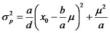
  constitute the portfolio frontier, whereas those above the minimum-variance portfolio constitute the efficient frontier. The variance of a portfolio as a function of
  is given by
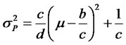 . (3)
. (3)
The traditional efficient frontier is illustrated in Figure 1.
3. Mean-Variance Model with a Cash Account
3.1. The Modified Model
The traditional mean-variance model does not reflect the fact that investors are able to keep a portion of their funds in the cash account. To accommodate this fact, the second constraint in model (1) should be relaxed as
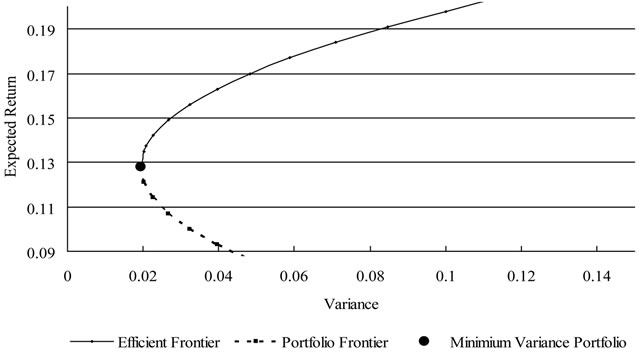
Figure 1. The traditional mean-variance efficient frontier.
 . If investors are able to borrow cash at a zero cost, then the constraint no longer exists. Accordingly, the mean-variance model becomes
 (4)
(4)
s.t. .
.
The cash account in this paper is defined as a banking account that pays no interest. Thus, cash provides a return of zero with no risk. Note that the cash account is assumed to be available to any investors, even though the investment opportunity set includes only n risky assets. This is in contrast with the risk-free asset considered in the traditional portfolio selection problem, as the riskfree asset is not available if it is not included in the opportunity set. Suppose the solution to model (4) is , then the proportion of total funds invested in risky assets is
 . If
. If , it means that investors allocate only a part of their total funds to risky assets, and
  of their total funds are retained in cash. In the case that
 , investors allocate all funds to risky assets, and portfolio
  coincides with portfolio
 . On the other hand, if
 , then investors borrow
  of their total funds and invest them, together with the original funds, in risky assets. Thus, the efficient portfolios determined by model (1) are typically no longer efficient according to model (4), indicating that the presence of the second constraint in model (1) leads to a loss in efficiency [14].
3.2. The Solution and Properties
Using the Lagrange multiplier approach, we obtain the first-order optimality condition for problem (4) as follows
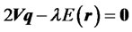 . (5)
. (5)
Solving for  from Equation (5) gives
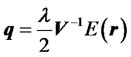 . (6)
. (6)
Plugging Equation (6) into the constraints in Equation (4) yields
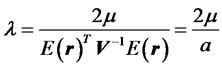 .
.
Therefore, the efficient portfolio for the given required return  in our model is
 . (7)
. (7)
Consequently, the proportion of total funds invested in risky assets is calculated as
 . (8)
. (8)
The following discussion considers the case in which . The cases of
  and
and  will be investigated in the last subsection.
Proposition 1. If the required return , then investors place only a part of their total funds in risky assets; if the required return
 , then investors invest their total funds in risky assets; if the required return
 , then investors borrow certain funds and invest them, together with their original amount, in risky assets.
Proof. It follows immediately from Equation (8).
Proposition 1 suggests that instead of investing all their funds in risky assets, investors will keep a part of their total funds in cash, as long as the required return is lower than the expected return on . This partially explains the general practice observed in the investment funds industry.
Next, we analyze how the portion of funds invested in risky assets is allocated among these risky assets in our model. According to Equations (7) and (8), the relative weights allocated in each of these assets are given
 . (9)
. (9)
Interestingly, the relative weights in the risky assets are the same as the weights of portfolio , regardless of the required return on the portfolio. Equations (8) and (9) yield
 . (10)
The intuition behind Equation (10) is that if , then investors only invest
  (percentage) of their total funds in portfolio
  and the rest
  is retained in cash. On the other hand, if
 , then investors borrow
  (percent) of their total funds and invest all these funds including the original amount in portfolio
 . This demonstrates that the efficient portfolios of risky assets under the modified mean-variance model are directly determined by the percentage (or times) of total funds in portfolio
 , while the rest is kept in cash (or borrowed). In other words, all funds will be allocated between portfolio
  and cash. This is the twofund separation theorem in our model, where the two funds are
  and the cash account.
It is believed that setting aside a certain amount of cash by fund managers may affect portfolio efficiency. However, our result indicates that this is not necessarily true. Portfolio efficiency depends on whether the portion of funds in risky assets is allocated in accordance with the relative weights of portfolio , and has nothing to do with whether or not certain funds are retained in the form of cash.
According to the new two-fund separation theorem, the portfolio selection process can be described as follows. First, for a given expected return, investors decide the proportion of their total funds invested in risky assets, the rest to be deposited in the cash account or borrowed. Second, investors allocate these funds among these risky assets according to the weights of portfolio . Therefore, all investors will hold the same risky portfolio regardless of risk aversion. Given that the market portfolio is the linear convex combination of portfolios of individual investors when the market is in equilibrium, portfolio
  is the market portfolio in the modified model.
For any given required return , the variance of the portfolio determined by Equation (7) is
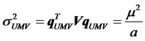 . (11)
 is the efficient frontier generated by the risky assets in the presence of a cash account. The minimumvariance portfolio is the one in which all funds are retained in cash with a return of zero.
3.3. The New Efficient Frontier versus the Traditional Efficient Frontier
To compare the efficient portfolios determined by model (4) with the efficient portfolios in the traditional model, we investigate their relative risks and Sharpe ratios for the same required return. From Equations (3) and (11), we note that
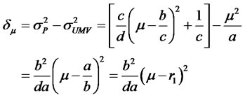 (12)
(12)
Given that  and
and ,
,  is always nonnegative, demonstrating the loss in efficiency of the traditional efficient portfolios relative to the new efficient portfolios. Namely, efficient portfolios determined by model (4) can achieve even lower risk than traditional efficient portfolios for any given required return that is not equal to
 . In addition, the bigger the difference between
  and
and , the greater the loss in efficiency of traditional efficient portfolios.
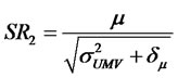
Assume without loss of generality that the risk-free rate is zero, then the Sharpe ratio of efficient portfolios determined by model (4) is given as
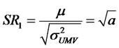 .
.
On the other hand, the Sharpe ratio of traditional efficient portfolios is
 .
.
Apparently,  is a constant, and is always greater than
  as long as the required return is not equal to
 .
.
Proposition 2. Portfolio  is the only portfolio on the traditional efficient frontier that also lies on the new efficient frontier determined by model (4), and all other traditional efficient portfolios are dominated by the corresponding new efficient portfolios for the given expected return. The traditional efficient frontier is innertangent to the efficient frontier determined by model (4) at point
 .
.
Given that both efficient frontiers are parabolas and that  is always non-negative, the traditional frontier must stay inside of the efficient frontier determined by model (4) with the only point of intersection
 . Thus, Proposition 2 follows immediately. Figure 2 displays the relation between these two efficient frontiers.
3.4. No Zero-Cost Borrowing
It is practically impossible to borrow funds at a zero cost.
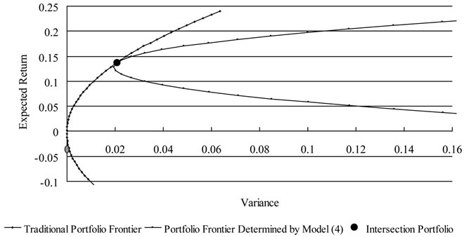
Figure 2. The traditional mean-variance efficient frontier and the efficient frontier determined by model (4).
If investors are not allowed to borrow, then the proportion of total funds in risky assets cannot exceed one, i.e., . To accommodate this restriction, model (1) becomes
 , (13)
s.t.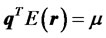 ,
,
 .
.
From Proposition 1, we notice that investors place a portion of their total funds in risky assets when , while they invest all their funds in risky assets when
 . In both cases, the no-borrowing restriction is satisfied, and models (13) and (4) imply the same portfolio decision.
However, when , the solution to model (4) violates the no-borrowing restriction. In this case, the decision implied by model (13) is consistent with the traditional mean-variance decision. To illustrate this point, we consider the following model:
 , (14)
s.t. ,
,
 .
.
In this model the proportion of total funds in risky assets is parameterized as  (
( ). The efficient frontier determined by model (14) is solved as
 . (15)
Equation (15) demonstrates that when  or
or ,
,  decreases with
  in the domain of
 . To achieve the minimum variance,
  must be maximized, or
 . As a result, the model reduces to the traditional mean-variance problem when
 , and yields the same decision as that in the traditional model.
Proposition 3. If borrowing is not allowed, then the efficient frontier is characterized by the following expression:
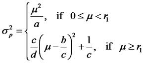 (16)
(16)
The solid line in Figure 3 displays the efficient frontier under this circumstance. Apparently, the portfolios determined by model (13) still perform at least as well as traditional efficient portfolios in terms of risk reduction.
3.5. b ≤ 0
When , the net funds in risky assets are negative according to Equation (8), indicating short-sales of risky assets. More specifically, investors will short sell portfolio and keep all the money in cash, regardless of whether or not borrowing is allowed. Moreover, the higher the required return, the more assets will be short-sold. In this case, the traditional efficient frontier is inner-tangent to the lower part of the portfolio frontier determined by the modified model.
In particular, when , the portfolios of risky assets are self-financing, and the traditional efficient frontier reduces to
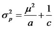 .
.
Therefore, the traditional efficient frontier of risky assets is located to the right of the efficient frontier determined by the modified model with the distance being .
.
4. A Numerical Analysis
Since the mean-variance model with a no-short-selling
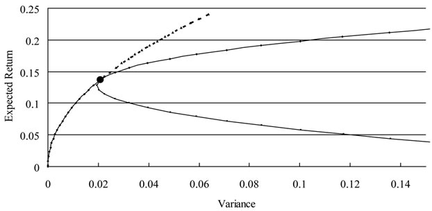
Figure 3. The traditional mean-variance efficient frontier and the efficient frontier determined by model (4) if borrowing is not allowed.
constraint cannot be solved analytically, our previous theoretical analysis does not impose the no-short-selling constraint. However, short-selling is difficult to implement in practice. This section begins by using a simulation to illustrate the performance of efficient portfolios determined by our model with the no-short-selling constraint relative to the traditional portfolios. Then, we demonstrate our theoretical findings using real data. To this end, we compare the following two groups of portfolios: the traditional minimum-variance portfolio (MVP) versus the efficient portfolio in the modified model with the same return as that on the MVP (EP0), as well as the equally-weighted portfolio (EWP) versus the efficient portfolios in both the traditional (EP1) and modified models (EP2) that generate the same return as does the EWP.
4.1. Data
The data used for the numerical analysis include the average value-weighted monthly returns on 10 industry portfolios in the US for the sample period from January 1976 to October 20101. These industry portfolios are constructed from all AMEX, NYSE and NASDAQ stocks by using their four-digit SIC codes from Compustat. Whenever Compustat SIC codes are not available, the CRSP SIC codes are taken. The data is obtained from Kenneth R. French’s personal website.
Table 1 reports the summary statistics of these portfolio returns. Apparently, NoDur and Enrgy yielded the highest returns, while HiTec and Durbl exhibited the highest risk over the past 30 years. Utils seems to be the safest industry among all 10 industries with the lowest return. In addition, the correlation coefficients between any pair of industry returns range from 0.26 to 0.84.
4.2. A Simulation
Our simulation is based on the results in Table 1. Denote the return vector obtained in Table 1 as  and variancecovariance matrix
 . Given these inputs, the portfolio weights are determined based on the traditional and modified models. To this end, we assume that the dynamics of returns follow a multi-variate standard normal distribution
 , and then simulate to obtain 10,000 realizations of each portfolio considered. The realized returns on each portfolio are used for our analysis. The major advantage of simulations is that there are no estimation errors, given the assumed data generating process, which allows for a fair comparison of portfolios under consideration. In addition, simulations enable us to examine cases in which analytic solutions are not available as well as gauge the percentage of funds in risky assets in the absence of estimation errors.
Table 2 reports the simulation results. We see that all the standard deviations of portfolios determined by our model are lower than those of corresponding traditional efficient portfolios, regardless of the type of portfolio, and thereby they have higher Sharpe ratios. We also find that the proportion of funds in portfolios determined by the modified model ranges from 0.8993 to 0.9322. Moreover, the model without a no-short-selling constraint induces a lower risky asset weight than the model with a no-short-selling constraint. Given that short-selling is typically not allowed in practice, our model implies that investors generally retain 6% to 9% of their funds in the cash account, while still being able to achieve expected returns that are as high as those on traditional efficient portfolios.
4.3. An Analysis Based on Real Data
The purpose of this section is to re-examine the issues in Section 4.2 with real data in terms of out-of sample performance.
4.3.1. The Test Design
To construct the minimum-variance portfolio, we need to first estimate the covariance matrix of risky assets. The sample covariance matrix,  is given by
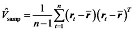 , (17)
where  is the vector of the arithmetic average of observed returns
  (
(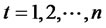 ). It is well documented that
  is an imprecise estimator of the true covariance matrix, and efficient portfolios based on this estimator perform poorly out of sample [15,16]. For this reason, we also consider shrinkage estimators and a combination of various estimators in addition to the sample covariance matrix. The rationale for the shrinking estimation method is that it shrinks the sample covariance matrix toward a lower-variance target, thereby reducing estimation errors and improving the out-of-sample performance.
The first shrinkage estimator considered is the one based on the single-factor model [17], which is denoted as . The second one, denoted as
 , is obtained by shrinking the sample covariance matrix toward the constant correlation matrix [18]. The final estimator
  is the simple average of the above three estimators, i.e.,
 . (18)
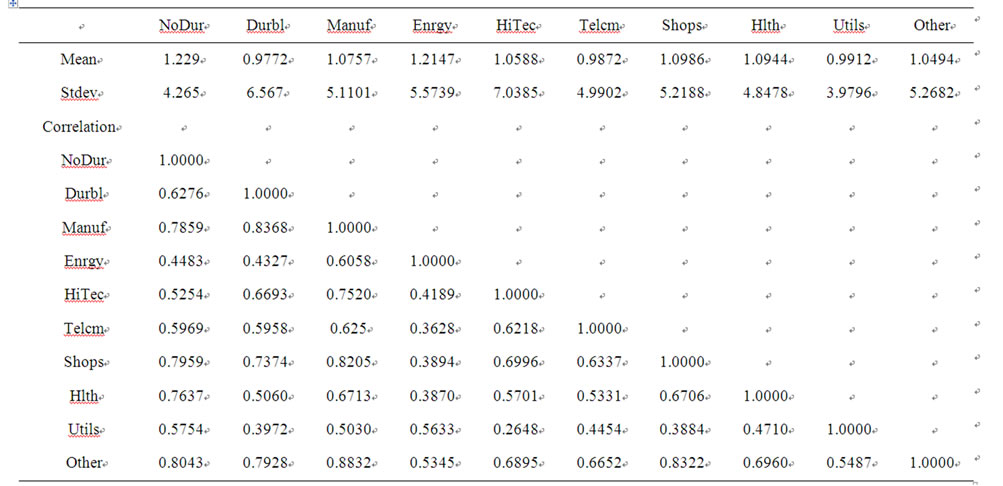
Table 1. Summary statistics of returns on industry portfolios.
This table reports mean returns, standard deviations, and correlations of the 10 US industry portfolios for the time period from January 1976 to October 2010.
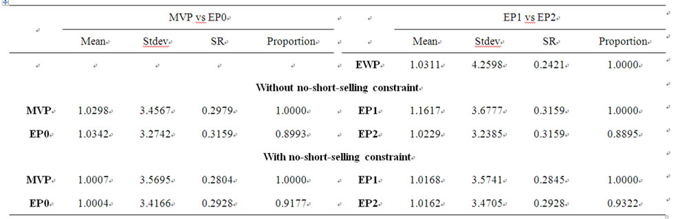
Table 2. Simulation results.
This table reports the mean, standard deviation (StdDev), and Sharpe ratio (SR) of each of the simulated portfolios. The proportions of total funds in risky assets in each case are also presented.
In this exercise, we also need to estimate the expected return vector to constructed efficient portfolios under the traditional and modified models. To this end, the sample means are used in the analysis.
Estimation errors arising from different estimation methods may greatly affect the portfolio’s out-of-sample performance. In addition to estimation methods, the sample size may also lead to estimation errors. For this reason, we consider cases in which parameters are calibrated from the most recent 120 and 240 monthly returns. To make it comparable under different scenarios, we start constructing portfolios from the 241st month based on the estimated inputs using different estimation methods and data sets, and reconstruct a new portfolio every month until the end of the sample period. The monthly returns of these portfolios are recorded and used for our analysis.
4.3.2. The Results
To assess portfolio performance, we calculate the outof-sample portfolio returns, standard deviations, and Sharpe ratios under different scenarios. The results are reported in Table 3.
. 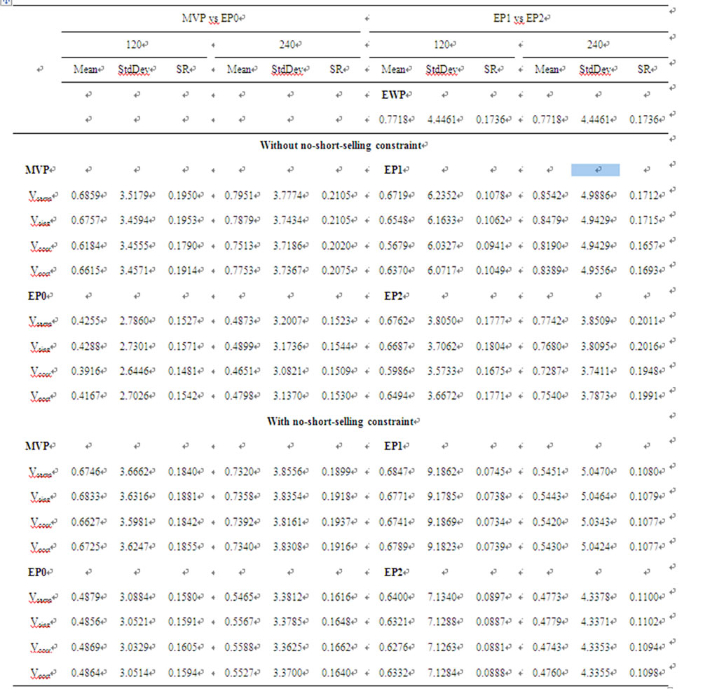
Table 3. Out-of-sample performance of traditional efficient portfolios and efficient portfolios determined by the modified model under various scenarios.
This table reports the out-of-sample means, standard deviations (StdDev), and Sharpe ratios (SR) of various portfolios under consideration for different estimation methods and sample sizes. Vsamp, Vsing, Vcorr, and Vport refer to cases when the covariance matrix is the sample covariance, shrinkage estimator based on the single factor model, shrinkage estimator based on the constant correlation, and a simple average of the above three estimators, respectively.
First, we notice that the EP0s are less risky than the MVPs, but generate lower mean returns and Sharpe ratios than does the MVP under different scenarios, regardless of whether or not the no-short-selling constraint is imposed. This result is primarily due to estimation errors. As we know, the MVP depends solely on the estimation of
the covariance matrix, while the EP0 depends on the estimation of both the covariance matrix and the mean returns of risky assets. Moreover, mean returns are more difficult to accurately estimate than the covariance matrix (Merton, 1972; Best and Grauer, 1991), and they have a larger impact on the portfolio weights than do the variances and covariances. Consequently, the improvement in the efficiency of the EP0s is largely offset by the imprecise return estimation.
Second, both the EP1 and EP2 portfolios generate similar out-of-sample mean returns, but the standard deviation of the EP2 is lower than that of the EP1. As a result, the EP2 typically has a higher Sharpe ratio than the EP1. This is not surprising, as both the EP1 and EP2 are now influenced by the estimation of both means returns and covariance matrix, and are thereby subject to the similar effect of estimation errors. Consistent with what the theoretical models predict, the efficient portfolio determined by our model is more efficient than the traditional efficient portfolio in terms of out-of-sample Sharpe ratios.
Third, we find that none of efficient portfolios EP0, EP1, and EP2 can beat the EWP in terms of the out-ofsample mean return, which is in line with the findings in the literature [19-22]. This is particularly pronounced when short-selling is not allowed. The EWP generates superior returns, because it avoids allocating most funds to assets that performed well in the past and few funds to assets that performed poorly, and thereby it is better diversified than efficient portfolios. Compared with efficient portfolios determined in either the traditional model or our model, the EWP places relatively high weights on smallcap assets and relatively low weights on large-cap assets. Therefore, the EWP can better capture the size effect and the Alpha return of small-cap stocks.
Finally, an increase in sample size helps improve portfolio performance, whereas the use of an advanced covariance estimation method does not seem to significantly improve portfolio performance. This is not surprising, given that there are only 10 industry portfolios in our dataset. Thus, when there are relatively few assets available, extending the estimation window is more effective in reducing the effect of estimation error than is adopting an advanced estimation method.
4.3.3. Portfolio Weights
To further explain our aforementioned observations, we investigate the proportions of total funds in risky assets determined by our model under different scenarios, which are plotted in Figure 4. We find that the longer the estimation window, the higher the weight placed in risky assets. In addition, the imposition of the no-short-selling constraint results in a higher proportion of total funds in risky assets than does the case of without a no-shortselling constraint. This explains why portfolios based on longer estimation periods and those with the no-shortselling constraint have higher standard deviations than those based on shorter estimation periods and without the no-short-selling constraint, observed in Table 3
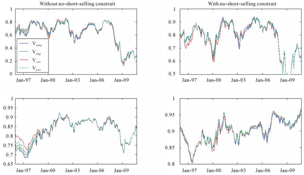
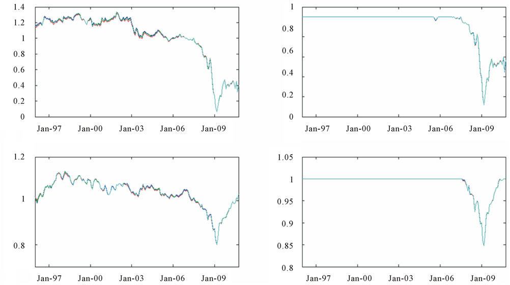
This figure plots the proportion of total funds in risky assets determined by the modified model under different scenarios. Panel A is for the efficient portfolio with the return equal to the return on the traditional minimum-variance portfolio, while Panel B is for the efficient portfolio with the return equal to the return on the equally-weighted portfolio. For each panel, the plots are for the cases of without no-short-selling constraint (left) and with no-short-selling constraint (right), and cases of when model inputs are estimated with sample sizes of 120 (top) and 240 (bottom).
From Figure 4, we can see that the proportion of funds in risky assets varies greatly over time, reflecting changes in market conditions. For example, during the bear market period from October 2007 to February 2009 in the US, the proportion implied by our model was reduced dramatically. This indicates that the efficient portfolios determined by our model are capable of limiting downside returns compared with the traditional efficient portfolios when the market is down. Under this circumstance, the cash account serves to hedge against the market risk. On the other hand, keeping part of funds in the cash account reduces the capability of obtaining high returns in the bull market. On average, the new efficient portfolios can generate returns as high as can the traditional efficient portfolios, but have a lower risk. As a result, the efficient portfolios determined in our model yield a higher Sharpe ratio than do the traditional efficient portfolios.
Interestingly, the plots in panel B indicate that the proportion of funds invested in risky assets is greater than 1 before the year 2006 if no restrictions are imposed. This is because the required return, which is equal to the return on the EWP, is higher than  during this time period. Accordingly, the efficient portfolio determined by our model coincides with the traditional efficient portfolio when the non-negative weight and non-borrowing restrictions are imposed.
5. Conclusions
The traditional mean-variance model requires that funds be fully invested in risky assets, which eliminates the possibility of keeping a part of funds in cash. This restriction distorts the efficient frontier and investors’ optimal portfolio decision. This paper investigates the meanvariance model in the presence of a cash account and examines properties of the efficient portfolios determined by this modified model. In addition, we conduct an empirical investigation to confirm our theoretical findings.
Our analysis shows that investors will keep a portion of their funds in cash as long as the required return is lower than the expected return of portfolio . In this case, the investment decision is about how to allocate funds between portfolio
  and the cash account. Further, the new efficient portfolios are more efficient than the traditional efficient portfolios. Our simulation results indicate that typically 6% to 9% of total funds are retained in cash if short-selling is not allowed, while these percentages are even higher if short-selling is possible. Based on the real data from the US over the past 30 years, we demonstrate that efficient portfolios determined by our model yield a higher out-of-sample Sharpe ratio than do traditional efficient portfolios. This is because our efficient portfolios are always less risky than traditional efficient portfolios, while still being able to generate returns similar to those from traditional efficient portfolios by limiting downside returns in the bear market.
6. Acknowledgements
Jiang and Ma acknowledge the support from National Natural Science Foundation of China (70932005) and Doctoral Programs Foundation of Ministry of Education of China (20100175110017); Jiang acknowledges the support from National Natural Science Foundation of China (71101019) and Fundamental Research Funds for the Central Universities in China (ZYGX2009J117). An acknowledges the support from the Odette School of Business at the University of Windsor.
REFERENCES
- H. Markowitz, “Portfolio Selection,” Journal of Finance, Vol. 7, No.1, 1952, pp. 77-91. doi:10.2307/2975974
- F. Black, “Capital Market Equilibrium with Restricted Borrowing,” Journal of Business, Vol. 45, No. 3, 1972, pp. 444-455. doi:10.1086/295472
- W. F. Sharpe, “Capital Asset Prices: A Theory of Market Equilibrium under Conditions of Risks,” Journal of Finance, Vol. 19, No. 3, 1964, pp. 425-442. doi:10.2307/2977928
- J. Lintner, “The Valuation of Risk Assets and the Selection of Risky Investments in Stock Portfolio and Capital Budgets,” Review of Economics and Statistics, Vol.47, No. 1, 1965, pp. 13-37. doi:10.2307/1926735
- J. Mossin, “Equilibrium in a Capital Asset Market,” Econometrica, Vol. 34, No. 4, 1966, pp. 768-783. doi:10.2307/1910098
- M. J. Brennan and Y. H. Xia, “Dynamic Asset Allocation under Inflation,” Journal of Finance, Vol. 57, No. 3, 2002, pp. 1201-1238.
- C. Jiang, Y. Ma and Y. An, “An Analysis of Portfolio Selection with Background Risk,” Journal of Banking and Finance, Vol. 34, No. 12, 2010, pp. 3055-3060. doi:10.1016/j.jbankfin.2010.07.013
- B. H. Solnik, “Inflation and Optimal Portfolio Choices,” Journal of Financial & Quantitative Analysis, Vol. 13, No. 5, 1978, pp. 903-925. doi:10.2307/2330634
- W. F. Sharpe, “Mutual Fund Performance,” Journal of Business, Vol. 39, No. 1, 1966, pp. 119-138. doi:10.1086/295080
- X. Cui, D. Li and J. Yan, “Classical Mean Variance Model Revisited: Pseudo Efficiency,” 2009. http://ssrn.com/abstract=1507453.
- R. Roll, “A Mean/Variance Analysis of Tracking Error,” Journal of Portfolio Management, Vol. 18, No. 4, 1992, pp. 13-22. doi:10.3905/jpm.1992.701922
- R. Merton, “An Analytical Derivation of the Efficient Portfolio Frontier,” Journal of Financial & Quantitative Analysis, Vol. 7, No. 4, 1972, pp. 1851-1872. doi:10.2307/2329621
- J. Tobin, “Liquidity Preference as Behaviour towards Risk,” Review of Economic Studies, Vol. 25, No. 2, 1958, pp. 65-86. doi:10.2307/2296205
- G. J. Alexander and A. M. Baptista, “Active Portfolio Management with Benchmarking: A Frontier Based on Alpha,” Journal of Banking and Finance, Vol. 34, No. 9, 2010, pp. 2185-2197. doi:10.1016/j.jbankfin.2010.02.005
- M. J. Best and R. R. Grauer, “On the Sensitivity of MeanVariance-Efficient Portfolios to Changes in Asset Means: Some Analytical and Computational Results,” Review of Financial Studies, Vol. 4, No. 2, 1991, pp. 315-342. doi:10.1093/rfs/4.2.315
- F. Black and R. Litterman, “Global Portfolio Optimization,” Financial Analysts Journal, Vol. 48, No. 5, 1992, pp. 28-43. doi:10.2469/faj.v48.n5.28
- O. Ledoit and M. Wolf, “Improved Estimation of the Covariance Matrix of Stock Returns with an Application to Portfolio Selection,” Journal of Empirical Finance, Vol. 10, No. 5, 2003, pp.603-621. doi:10.1016/S0927-5398(03)00007-0
- O. Ledoit and M. Wolf, “Honey, I Shrunk the Sample Covariance Matrix,” Journal of Portfolio Management, Vol. 30, No. 4, 2004, pp. 110-119.
- V. DeMiguel, L. Garlappi and R. Uppal, “Optimal versus Naive Diversification: How Inefficient Is the 1/N Portfolio Strategy?” Review of Financial Studies, Vol. 22, No. 5, 2009, pp. 1915-1953. doi:10.1093/rfs/hhm075
- R. Duchin and H. Levy, “Markowitz versus the Talmudic Portfolio Diversification Strategies,” Journal of Portfolio Management, Vol. 35, No. 2, 2009, pp. 71-74. doi:10.3905/JPM.2009.35.2.071
- J. Fletcher, “Risk Reduction and Mean-Variance Analysis: An Empirical Investigation,” Journal of Business Finance & Accounting, Vol. 36, No. 7-8, 2009, pp. 951-971. doi:10.1111/j.1468-5957.2009.02143.x
- M. Kritzman, S. Page and D. Turkington, “In Defense of Optimization: The Fallacy of 1/N,” Financial Analyst Journal, Vol. 66, No. 2, 2010, pp.31-39. doi:10.2469/faj.v66.n2.6
NOTES
1These portfolios include NoDur (consumer non-durables), Durbl (consumer durables), Manuf (Manufacturing), Enrgy (oil, gas, and coal extraction and products), HiTec (business equipment), Telcm (telephone and television transmission), Shops (wholesale, retail, and some services), Hlth (healthcare, medical equipment, and drugs), Utils (utilities), and Other.