Open Journal of Statistics
Vol.07 No.04(2017), Article ID:78250,13 pages
10.4236/ojs.2017.74042
Assessing Actuarial Projections Accuracy: Traditional vs. Experimental Strategy
Maria Russolillo
Department of Economics and Statistics, University of Salerno, Fisciano, Italy
![]()
Copyright © 2017 by author and Scientific Research Publishing Inc.
This work is licensed under the Creative Commons Attribution International License (CC BY 4.0).
http://creativecommons.org/licenses/by/4.0/


Received: July 5, 2017; Accepted: August 6, 2017; Published: August 9, 2017
ABSTRACT
This paper gives an overview of the Lee Carter method and reiterates the feasibility of using it to construct mortality forecast for the population data. In a first step, the model is fitted in a traditional way and used to extrapolate forecast of the time-varying mortality index. The observed pattern of the mortality rates shows a different variability at different ages, highlighting that the homoscedasticity hypothesis is quite unrealistic. Thus, in a second step, the paper aims to produce more reliable mortality forecasting, focusing on the errors in the estimation of the model parameters. The robustness of the estimated parameter is analysed throughout an experimental strategy which allows to assess the robustness of the Lee Carter model by inducing the errors to satisfy the homoscedasticity hypothesis. The graphical and numerical results are tested by means of a comparison in terms of prediction accuracy.
Keywords:
Lee-Carter Model, Singular Value Decomposition, Experimental Strategy, Mortality Projections, Life Expectancy at Birth

1. Introduction
The actuarial literature has developed a number of approaches to make objective projections on mortality rates [1] [2] [3] . In particular, in the last decades, actuaries and demographers have made increasing use of more and more sophisticated methods to forecast mortality. They moved towards stochastic methods, which have the advantage of producing a forecast probability distribution rather than a deterministic point forecast. Among the others, we focus on extrapolative methods of mortality forecasting, which make use of the regularity typically found in both age patterns and trends over time to extrapolate aggregate measures such as life expectancy in a traditional and relatively simple way. Belong to these methods the Lee Carter (LC hereinafter) method becomes popular thanks to its practical applicability, accuracy and objectivity of the results. This model, introduced by Lee and Carter in 1992 [4] , has become a landmark in the demographic literature. It combines the information about mortality level and age pattern to explain the observed mortality rates. However, the model has quite stringent assumptions and some defects. One of the assumptions is that the age factor is constant to time factor, but this will determine a loss of ability to reflect the mutual effect between age and time. Traditional LC model needs large data size, but this requirement cannot be satisfied by all the countries. Another typical assumption is that the errors are homoscedastic. We will deal with this hypothesis which can seriously differ from reality. In the last few years many researchers have proposed models to improve the LC model, even if in many cases they lost advantages in simplicity and effectiveness in fitting accuracy. Some authors, for example, added variables to put birth-year effect into the model [5] , but they found multicollinearity and homoscedasticity. Other authors have combined other theories trying to expand the utility of the model, without improving model effect, but making the model much more complicated. For this reasons, we choose to focus on the basic LC model, with the aim to take into account the more realistic hypothesis of homoscedasticity in the errors. In particular, once we have tested that errors show homoscedasticity, we propose an experimental strategy to assess the robustness of the LC model by inducing the errors to satisfy the homoscedasticity hypothesis. Final aim of the paper is to show that, by considering the homoscedasticity in the errors, it is possible to obtain more reliable mortality projections. The paper is structured as follows: in Section 2, we give a brief overview of the LC model, its fitting using Singular Value Decomposition and the Iterative procedure to estimate the time-varying parameter. In Section 3, we develop an experimental strategy to face the homoscedastic issue of the LC model. In Section 4, an application to real data is illustrated using Italian mortality rates and the performance of our experiment is examined by a comparative study. Some concluding remarks are provided in Section 5.
2. About the Lee Carter Model
Let us recall the traditional LC model analytical expression (4):
(1)
where are the log-mortality rates and , and are an age-spe- cific parameter independent of time, a coefficient describing the tendency of mortality to change and a time-varying parameter, respectively. The error term is assumed to be homoscedastic (with mean 0 and variance ).
2.1. Fitting the Model Using Singular Value Decomposition
To find a Least Squares Solution to the LC analytical expression, we use the close approximation to the Singular Value Decomposition (SVD) method proposed by Lee and Carter [4] , initially assuming that the errors are homoscedastic. To obtain a unique solution, the sum of the coefficients is fixed equal to 1 and the sum of the parameters equal to 0. The SVD approximation follows the next step:
1) We estimate as the logarithm of the geometric mean of the crude mortality rates, averaged over all , for each :
In other words, the coefficients must be simply the average values over time of the values for each .
2) We compute as the sum over age of .
3) We estimate from (where refers to the estimated at step 2) using the least squares estimation, i.e. choosing
to minimize Math_26#.
By way of these steps, we find each by regressing on , without a constant term, separately for each age group .
2.2. The Iterative Procedure to Estimate kt
The estimation introduced in Section 2.1, is a first stage estimation based on logs of death rates rather than the death rates themselves. To guarantee that the fitted death rates will lead to the actual numbers of deaths, when applied to given population age distribution, it is necessary to estimate in a second step, taking the and estimates from the first step. In particular, we use an iterative method to adjust the estimated , so that the actual total observed deaths
equal the total expected deaths , for each year .
The iterative method proceeds as follows:
1) We compare the total expected deaths to the actual total observed deaths in each period.
2) With this comparison, we can find one of three possible states:
i) If , we need to decrease the expected deaths, adjust-
ing the estimated so that the new estimate of , say , will be: , if (where is the first estimate of ); , if , where is a small number.
ii) If , we stop here the iterations.
iii) If , we need to increase the expected deaths adjusting
the estimated so that : , if ; , if .
3) Go back to Step 1.
Once we obtain the new time-varying parameter , we can model it as a stochastic process. To this aim, we use the standard Box and Jenkins methodology (identification-estimation-diagnosis) and choose an appropriate ARIMA (p, d, q) model for the mortality index [6] [7] .
3. The Homoscedasticity Issue: Designing the Experiment
Let us state with the matrix holding the mean centred log-mortality rates, given by . We can express the LC model as follows:
(2)
We have seen that, in the original LC model, the errors are supposed to be homoscedastic with respect to the different age-groups. This hypothesis can be seriously different from reality and can affect the robustness of the mortality index . As we know (4, Appendix B), the LC model incorporates different sources of uncertainty: uncertainty in the demographic model and uncertainty in forecasting. The uncertainty in the demographic model can be incorporated by considering errors in fitting the original matrix of mortality rates, while forecast uncertainty arises from the errors in the forecast of the mortality index. Aim of this contribution is to take into consideration the demographic component in order to focus on the sensitivity of the estimated mortality index. To achieve this aim, we propose an experimental strategy to force the fulfilment of the homoscedasticity hypothesis and to assess its effect on the LC estimates.
To induce the errors to satisfy the homoscedasticity hypothesis, we propose the following scheme:
1) We express the residual term as the difference between the matrix , referring to the mean centred log-mortality rates and the product between βx and kt, deriving from the LC model estimation:
(3)
2) We explore the residuals by means of statistical indicators such as: Range, Interquartile Range, Mean Absolute Deviation (MAD) of a sample of data, Standard Deviation, Box-plot, etc., in order to find some non-conforming age- groups.
3) We find those age-groups which show higher variability in the errors and rank the non-conforming age-groups according to decreasing non-conformity, i.e. from the more widespread to the more homogeneous one.
4) For each selected age-group:
4.1) we reduce the variability dividing the entire range in several quantiles, leaving aside each time the fixed α% of the extreme values;
4.2) we substitute the extreme values with uniform random values ranging from the αth to the 100-αth percentiles, with α given by: 0.05; 0.10; 0.15; 0.20; 0.25; 0.30.
5) For each age-group and for each percentile, we define a new error matrix which is used for computing a new data matrix , from which it is possible to derive the correspondent .
6) We replicate each running under the same conditions a large number of times (i.e.: 1000).
By way of this experiment, we investigate the residuals heteroscedasticity deriving from two factors: the age-group effect and the amount of altered values in each age-group. Throughout the successive running, we obtain more and more homogeneous error terms, which allow to determine the hypothetical pattern of . Thus, under these assumptions, we investigate the changes in which can be derived from every simulated error matrix.
From the relation:
(4)
we obtain a new matrix , where is the matrix holding the actual data and the matrix holding the mean of altered errors. Assuming fixed the βx, the are obtained as the Ordinary Least Square (OLS) coefficients of a multivariate regression model:
4. Numerical Application
4.1. Traditional LC
We fit the LC model to a data matrix of male Italian death rates, supplied by the Human Mortality Database [8] . The data, downloaded from year 1950 to 2000, are divided in 21 subgroups for five-year age groups, ranging from 0, 1 - 4 up to 95 - 99. We denote the “Death rates” by a matrix, where the first number refers to the age interval and the second number to the time interval. For each calendar year: , with , we consider all the ages , grouped in classes as . Following the SVD approximation described in Section 2.1, we obtain the raw estimates of , and . To eliminate potential differences between predicted and actual deaths, we run the iterative process described in Section 2.2 many times (1000) obtaining more reliable estimates.
We model the new time-varying parameter , as a stochastic process, following the standard Box and Jenkins methodology (identification-estimation- diagnosis). In a first step, we analyse the general pattern of the time series, noticing a decreasing linear trend (see Figure 1).
By using the Akaike and Schwarz Information Criterion (AIC and SIC) per model, together with examination of autocorrelations and partial autocorrelations, we select an ARIMA (0, 1, 0) process to model the male index, i.e.:
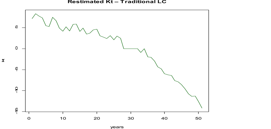
Figure 1. Mortality index trend―Traditional LC.

Table 1. ARIMA Model Coefficient.
In Table 1 are displayed the estimated parameters for the constant terms , indicating the average annual change of , with its standard errors. The moving average term and the autoregressive parameter are equal to zero in the ARIMA (0, 1, 0) case.
Basing on the period 1950-2000, we make use of the ARIMA (0, 1, 0) model to forecast the index of mortality for the next 25 years. The results will be compared in the next to the forecast derived by the experimental strategy.
4.2. Experimental LC
As explained in the previous section, the typical result of applying the LC model is a time series indicating the mortality trend. Figure 1 shows the estimates obtained from real data. With the experiment we propose, we aim to explore in which way the presence of heteroscedasticity can affect the successive forecasting process.
Following the scheme of our procedure, after expressing the error term as the difference: , we carry on an analysis of the residuals’ variability in order to find some “non-conforming” age-groups. We explore the residuals by means of some dispersion indices, in the matter in question Interquartile Range, MAD, Range and Standard Deviation, to determine the age-groups in which the model hypothesis does not hold (Table 2).
In Table 2, we highlighted in red the suspected age-groups, noticing that the
Table 2. The analysis of the residuals’ variability.
residuals in the age-groups 1 - 4; 5 - 9; 15 - 19 and 25 - 29 show the highest variability. The age - groups 30 - 34; 40 - 44; 50 - 54 could also be suspected and should be examined. To choose the age-groups to enter in our experiment, we provide also a graphical analysis. In Fig. 2 we display the boxplot of the residuals’ variability for each age-group in order to see if these residuals are in compliance with the expected ones.
If we have a look at the age-group 1 - 4; 15 - 19, which show the largest widespread, we can notice that the range goes from −2 to 2. We rank these non- conforming age-groups according to decreasing non-conformity, i.e. from the more widespread to the more homogeneous one. The ultimate aim is to analyze at what extend the estimated ’s are affected by such a variability.
On the basis of the previous analysis, we conclude that the age-groups 1 - 4; 5 - 9; 15 - 19 and 25 - 29 are far away from being homogeneous and will be sequentially entered in the experiment. For each of the four age-groups, we reduce the variability dividing the entire range into 6 quantiles: 5%, 10%, 15%, 20%, 25%, 30%, leaving aside each time a fixed 5% of the extreme values. We generate
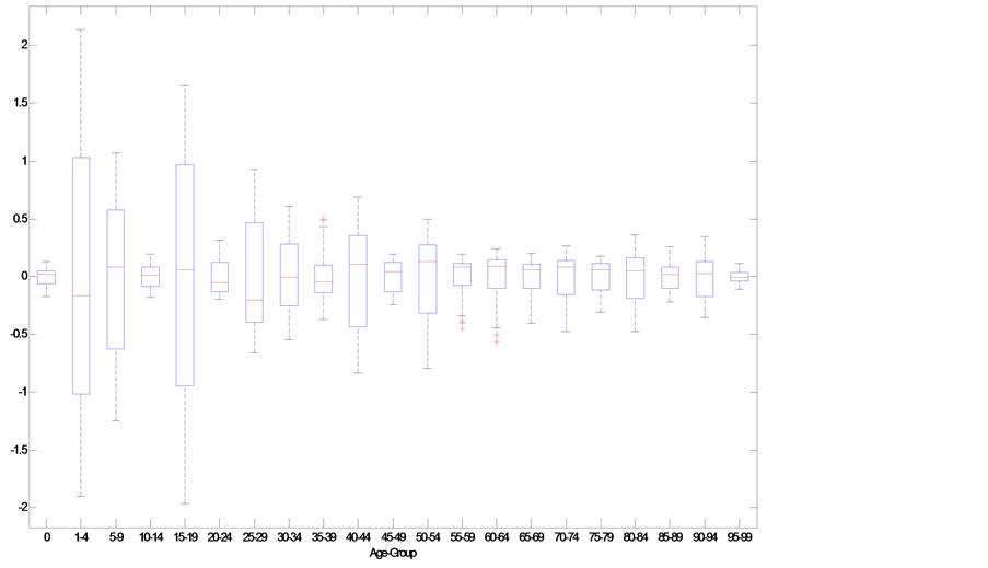
Figure 2. Residuals’ variability Boxplot for each age-group.
![]()
Figure 3. Plot-Matrix showing the Kt resulting from different experimental conditions.
1000 random replications and define, for each age-group and for each quantile, a new error matrix used for computing a new data matrix. From the replicated errors, we compute the estimated and then we extrapolate the 24 average of the 1000 simulated (Figure 3).
Figure 3 shows the 24,000 estimated (1000 Replications times 4 Age- groups times 6 quantile) arranged in 4 rows, representing the successive age- groups entered in the experiment, and the 6 columns representing the successive increment in the percentage of outer values which have been transformed. For better interpret this outcome, in Figure 4 we have plotted the resulting average of the 1000 under the 24 conditions.
By comparing the 24 averaged (in red) to the original one (in black), we can see the effect of the changes in homogeneity on the for each of the four age-groups. In particular, we can notice that as the homoscedasticity in the errors increases, ’s tend to be flatter than the original one. In other words, more regular residuals lead to a flatted pattern of the ’s. For sake of comparison, in Figure 5 we have matched in a Boxplot the original and transformed Residuals.
![]()
Figure 4. kt synthetic view.
![]()
Figure 5. Final versus Actual Residuals.
![]()
Figure 6. Response Surface.
In Figure 5, we can see that the final residual matrix (bottom row) shows, after the experiment, a more homogenous pattern in line with the classical hypothesis and varies in a range from −1 to 1. Finally, to better interpret the changes in the slope, in Figure 6 we illustrate the Response Surface [9] plotted for the four age-groups considered in the experiment. What is evident from the graph is that the more homogenous the residuals are, the more flatten the is.
4.3. Comparing Actuarial Projections
Our aim is to compare the results obtained from the LC model fitted in a traditional way to the results obtained processing the residuals with the proposed experimental strategy. In the last case, our findings showed that a more regular residual matrix leads to a flatter . Taking into consideration the new (let’s call it “experimental ”), our aim is to find an appropriate ARIMA time series model for the mortality index and then use that mortality model to generate forecasts of the mortality rates. The ultimate purpose is to compute life expectancy at birth from forecasted mortality rates in both cases and compare them to the actual one.
As first step, by following the methodology illustrated in Section 4.1, we find that, among the others, an ARIMA (0, 1, 0) model is more feasible for the experimental series as happened for the series derived from the traditional LC model (let’s call it “traditional ”). The ARIMA (0, 1, 0) models are then used to generate forecasts of the mortality index for the next 25 years based on the period 1950-2000. Table 3 lists these values for both cases.
As second step, we build up projected life tables in both cases, by using the traditional and experimental . The procedure tracked is the following: after
Table 3. ARIMA (0, 1, 0): Experimental versus traditional projected kt.
obtaining the projected series, we construct projected mortality rates. Then we project life expectancy at birth from 2001 up to 2009, by using the traditional in the first case and, for the same period, by using the experimental . In order to test the validity of our experiment, we compare the resulting life expectancy to the actual life expectancy at birth from 2001 up to 2009. The choice of the period (2001-2009) as the forecast date was due to the consideration of updated projections available for Italy in the HMD. Figure 7 shows the results in the three cases. This comparative analysis of the traditional and experimental procedure to the actual life expectancy values confirms satisfying results.
From Figure 7, we can notice that the experimental strategy we proposed leads to life expectancy values, which interpolates the actual ones. This result seems to confirm our initial hypothesis about the heteroscedasticity in the
![]()
Figure 7. Traditional, experimental and actual life expectancy at birth.
errors. In other words, if we take into account the heteroscedasticity in the errors, we obtain more realistic and reliable survival projections.
5. Conclusions
The LC mortality forecasting approach has several appreciated properties, but also quite stringent assumptions. A major one considers the errors homoscedastic but, in our experience, this is seriously different from reality. Our analysis illustrates the potential utility of considering the homoscedasticity issue of the LC model in survival analysis. When homoscedasticity is found in the residuals, we warn that successive forecast could be biased in some way. For this reason, what we propose is an experimental strategy to force the fulfilment of the homoscedasticity hypothesis by inducing the errors to satisfy it. In the numerical application we find that a more regular residual matrix leads to a more flat . We test this result by means of a comparison in terms of prediction accuracy. We project life expectancy at birth from 2001 up to 2009, by using the traditional , the experimental and comparing them to the actual life expectancy at birth projected for the same period. In terms of predictive performance, for this particular data set, we found that the experimental led to more realistic survival projections. In future research we would like to provide a statistical meaning in the sloping changes and to provide a general rule in assessing the LC model sensitivity.
Acknowledgements
The author thanks an anonymous referee whose suggestions improved the original manuscript.
Cite this paper
Russolillo, M. (2017) Assessing Actuarial Projections Accuracy: Traditional vs. Experimental Strategy. Open Journal of Statistics, 7, 608-620. https://doi.org/10.4236/ojs.2017.74042
References
- 1. Russolillo, M., Giordano, G. and Haberman, S. (2011) Extending the Lee-Carter Model: A Three-Way Decomposition. Scandinavian Actuarial Journal, 2, 96-117.
- 2. Li, N., Lee, R. and Gerland, P. (2013) Extending the Lee-Carter Method to Model the Rotation of Age Patterns of Mortality Decline for Long-Term Projections. Demography, 50, 2037-2051. https://doi.org/10.1007/s13524-013-0232-2
- 3. Haberman, S., Ed. (2014) Actuarial Methods. In: Wiley StatsRef: Statistics Reference Online, John Wiley & Sons, New York. https://doi.org/10.1002/9781118445112.stat06074
- 4. Lee, R.D. and Carter, L.R. (1992) Modelling and Forecasting U.S. Mortality. Journal of the American Statistical Association, 87, 659-671.
- 5. Renshaw, A. and Haberman, S. (2006) A Cohort-Based Extension to the Lee-Carter Model for Mortality Reduction Factors. Insurance: Mathematics and Economics, 38, 556-570. https://doi.org/10.1016/j.insmatheco.2005.12.001
- 6. Box, G.E.P. and Jenkins, G.M. (1976) Time Series Analysis for Forecasting and Control. Holden-Day, San Francisco.
- 7. Hamilton, J.D. (1994) Time Series Analysis. Princeton University Press, Princeton, NJ.
- 8. Human Mortality Database (2014) University of California, Berkeley (USA), and Max Planck Institute for Demographic Research (Germany). http://www.mortality.org/ http://www.humanmortality.de/
- 9. Box, G.E.P. and Draper, N.R. (1987) Empirical Model Building and Response Surfaces. John Wiley & Sons, New York.