Open Journal of Statistics
Vol.06 No.02(2016), Article ID:65869,12 pages
10.4236/ojs.2016.62023
Distribution of the Maximum and Minimum of a Random Number of Bounded Random Variables
Jie Hao1, Anant Godbole2
1Department of Statistics and Analytical Sciences, Kennesaw State University, Kennesaw, USA
2Department of Mathematics and Statistics, East Tennessee State University, Johnson City, USA

Copyright © 2016 by authors and Scientific Research Publishing Inc.
This work is licensed under the Creative Commons Attribution International License (CC BY).
http://creativecommons.org/licenses/by/4.0/


Received 28 January 2016; accepted 23 April 2016; published 26 April 2016
ABSTRACT
We study a new family of random variables that each arise as the distribution of the maximum or minimum of a random number N of i.i.d. random variables X1, X2, ∙∙∙, XN, each distributed as a variable X with support on [0, 1]. The general scheme is first outlined, and several special cases are studied in detail. Wherever appropriate, we find estimates of the parameter θ in the one-parameter family in question.
Keywords:
Maximum and Minimum, Random Number of i.i.d. Variables, Statistical Inference

1. Introduction
Consider a sequence  of i.i.d. random variables with support on
  and having distribution function F. For any fixed n, the distributions of

and

have been well studied; in fact it is shown in elementary texts that  and
and . But what if we have a situation where the number N of Xi’s is random, and we are instead considering the extrema
 (1)
(1)
and
 (2)
(2)
of a random number of i.i.d. random variables? Now the sum S of a random number of i.i.d. variables, defined as

satisfies, according to Wald’s Lemma [1] , the equation

provided that N is independent of the sequence  and assuming that the means of X and N exist.
The purpose of this paper is to show that the distributions in (1) and (2) can be studied in many canonical cases, even if N and  are correlated. The main deviation from the papers [2] [3] and [4] , where similar questions are studied, is that the variable X is concentrated on the interval
 ―unlike the above references, where X has lifetime-like distributions on
 . Even then, we find that many new and interesting distributions arise, none of them to be found, e.g., in [5] or [6] via the “extreme values of a random number of i.i.d. variables” connection. See, however, Remarks 1 and 2 in Section 3. In another deviation from the theory of extremes of random sequences (see, e.g., [7] ), we find that the tail behavior of the extreme distributions is not relevant due to the fact that the distributions have compact support. We next cite three examples where our methods might be useful. First, we might be interested in the strongest earthquake in a given region in a given year. The number of earthquakes in a year, N, is usually modeled using a Poisson distribution, and, ignoring aftershocks and similarly correlated events, the intensities of the earthquakes can be considered to be i.i.d. random variables in
  whose distribution can be modeled using, e.g., the data set maintained by Caltech at [8] . Second, many “small world” phenomena have recently been modeled by power law distributions, also sometimes termed discrete Pareto or Zipf distributions. See, for example, the body of work by Chung and her co-authors [9] [10] , and the references therein, where vertex degrees
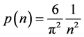
  in “internet-like graphs” G (e.g., the vertices of G are individual webpages, and there is an edge between v1 and v2 if one of the webpages has a link to the other) are shown to be modeled by

for some constant , where
  is the Riemann Zeta function

Thus if the vertices v in a large internet graph have some bounded i.i.d. property Xi, then the maximum and minimum values of Xi for the neighbors of a randomly chosen vertex can be modeled using the methods of this paper. Third, we note that N and the Xi may be correlated, as in the CSUG example (studied systematically in Section 3) where  and
and  follows the geometric distribution
 . This is an example of a situation where we might be modeling the maximum load that a device might have carried before it breaks down due to an excessive weight or current. It is also feasible in this case that the parameter θ might be unknown.
Here is our general set-up: Suppose  are i.i.d. random variables following a continuous distribution on
  with probability density and distribution functions given by
  and
and  respectively. N is a random variable following a discrete distribution on
  with probability mass function given by
 ,
, . Let Y and Z be given by (1) and (2) respectively. Then the p.d.f.’s g of Y and Z are derived as follows: Since

we see that

and consequently, the marginal p.d.f. of Y is
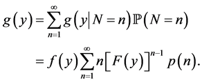 (3)
(3)
In a similar fashion, the p.d.f. of Z can be shown to be
 (4)
(4)
what is remarkable is that the sums in (3) and (4) will be shown to assume simple tractable forms in a variety of cases.
We want to point out that some of our distributions have been studied before but not using this motivation. For example, the Marshall-Olkin distributions [11] give a new method of adding a parameter to a distribution. Also, other distributions such as the beta and Kumaraswamy [12] distributions can be used to model continuous bounded data, but these do not apply to our set-up. See also Remark 2 in Section 3.
Our paper is organized as follows. Section 1 provided a summary and motivation for studying the distributions in the fashion we do. In Section 2, we study the case of  and
and . We call this the Standard Uniform Geometric model. The graphs of g(y) and g(z) can be seen in Figure 1 and Figure 2 respectively. The CSUG (Correlated Standard Uniform Model) is studied in Section 3. The graphs of g(y) and g(z) in the CSUG model are plotted in Figure 3 and Figure 4 respectively. Parameter estimation is done in Section 4. Section 5 is devoted to a summary of a variety of other models.
2. Standard Uniform Geometric (SUG) Model
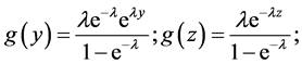
Since ,
,  , and
, and  for some
 , we have from (3) that the p.d.f. of Y in the SUG model is given by
 (5)
(5)
Similarly, (4) gives that
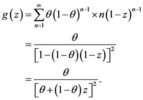 (6)
(6)
Proposition 2.1. If the random variable Y has the “SUG maximum distribution” (5) and , then
 Proof.
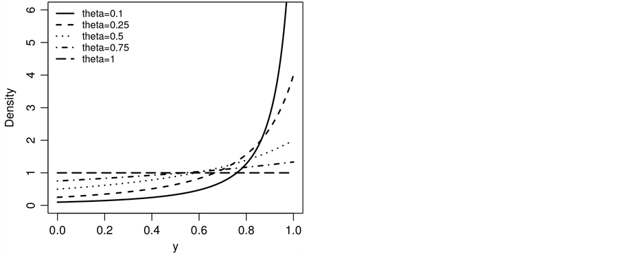
Figure 1. Plot of the SUG maximum density for some values of θ (see Equation (5)).
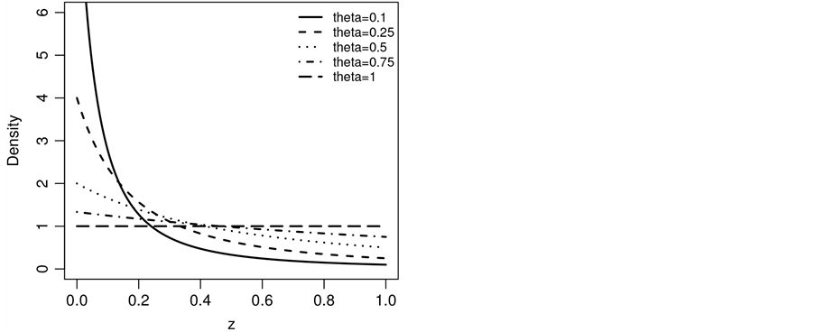
Figure 2. Plot of the SUG minimum density for some values of θ (see Equation (6)).
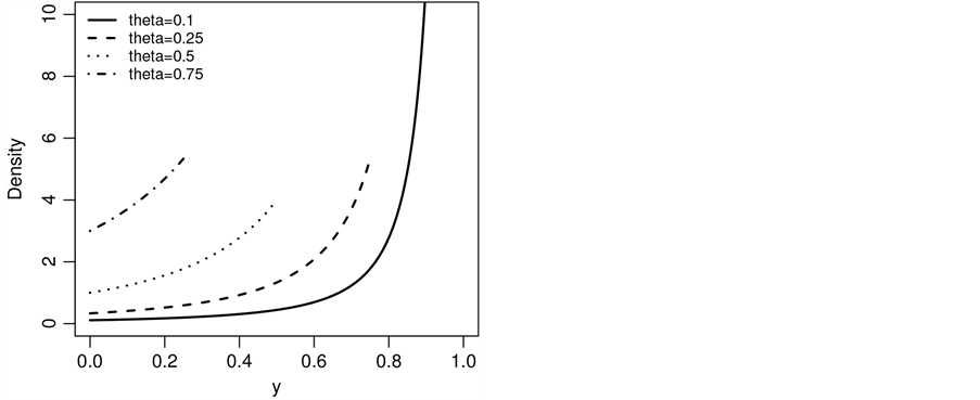
Figure 3. Plot of the CSUG maximum density for some values of θ.
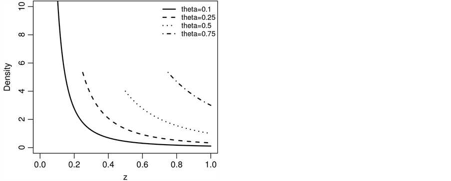
Figure 4. Plot of CSUG minimum density for some values of θ.
as claimed. □
Note. Even though we take the distributions to have support on , this may be done by changing the survival function in [3] , where the same compounding method is used. Specifically we can use the transformation
  in the proofs of [3] .
Proposition 2.2. The random variable Y has mean and variance given, respectively, by

Proof. Using Proposition 2.1, we can directly compute the mean and variance by setting , and using the fact that
  for any random variable W. (This proof could equally well have been based on calculating the moments of
  and then recovering the values of
  and
and . The same is true of other proofs in the paper.) □
Proposition 2.3. If the random variable Z has the “SUG minimum distribution” and , then

Proof.
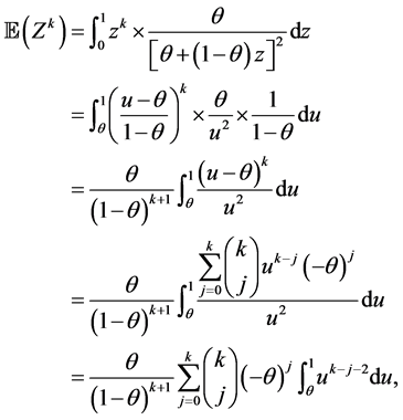
as asserted. □
Proposition 2.4. The random variable Z has mean and variance given, respectively, by

Proof. Using Proposition 2.3, it is easily to compute the mean and variance by setting k = 1, k = 2. □
The m.g.f.’s of Y, Z are easy to calculate too. Notice that the logarithmic terms above arise due to the contributions of the j = 1 and  terms, and it is precisely these logarithmic terms that make, e.g., method of moments estimates for θ to be intractable in a closed (i.e., non-numerical) form. Similar difficulties arise when analyzing the likelihood function and likelihood ratios.
3. The Correlated Standard Uniform Geometric (CSUG) Model
The Correlated Standard Uniform Geometric (CSUG) model is related to the SUG model, as the name suggests, but X and N are correlated as indicated in Section 1. The CSUG problems arise in two cases. One case is that we conduct standard uniform trials until a variable Xi exceeds , where θ is the parameter of the correlated geometric variable, and the maximum of
  is what we seek. The maximum is between 0 and
 . The other case is where standard uniform trials are conducted until Xi is less than θ, and we are looking for the minimum of
 . The minimum is between θ and 1.
Specifically, let  be a sequence of standard uniform variables and define

or

In either case N has probability mass function given by
 (7)
(7)
note that this is simply a geometric random variable conditional on the success having occurred at trial 2 or later. Clearly N is dependent on the X sequence.
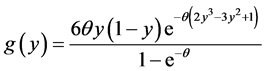
Proposition 3.1. Under the CSUG model, the p.d.f. of Y, defined by (1), is given by

Proof. The conditional c.d.f. of Y given that  is given by

Taking the derivative, we see that the conditional density function is given by

Consequently, the p.d.f. of Y in the CSUG model is given by
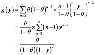
This completes the proof. □
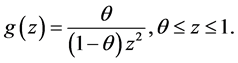
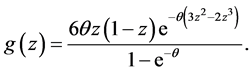
Proposition 3.2. The p.d.f. of Z under the CSUG model is given by
Proof. The conditional cumulative distribution function of Z given that  is given by

Thus, the conditional density function is given by

which yields the p.d.f. of Z under the CSUG model as
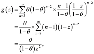
which finishes the proof. □
Proposition 3.3. If the random variable Y has the “CSUG maximum distribution” and , then

Proof.
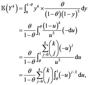
as claimed. □
Proposition 3.4. The random variable Y has mean and variance given, respectively, by

and

Proof. Using Proposition 3.3, we can directly compute the mean and variance by setting k = 1, 2. For example with k = 1 we get

Notice that the variance of Y is smaller than that of Y under the SUG model, with an identical numerator term. Also, the expected value is smaller under the CSUG model than in the SUG case. This can be best seen by the inequalities

and

valid for . □
. □
Proposition 3.5. If the random variable Z has the “CSUG Minimum distribution” and , then

Proof. Routine, as before. □
Proposition 3.6. The random variable Z has mean and variance given, respectively, by

and

Proof. A special case of Proposition 3.3; note that as in the SUG model, . □
. □
Remark 1. The four distributions of Y and Z under the SUG and the CSUG models can be shown to be affine transformations of the same distribution as seem by the following results (proofs omitted):
Proposition 3.7. Changing the variable Y of (5) as  yields (6). Thus the SUG maximum and SUG minimum variables are related by the fact that

Proposition 3.8. Changing the variable Y of the CSUG model (in Proposition 3.1) as  yields
 , which equals the pdf of (5). Hence

Proposition 3.9. Changing the variable Z of the CSUG model (in Proposition 3.2) as  yields
 , which equals the pdf of (6). Thus

As a result of these affine transformations, the moment equations (Propositions from 2.1 to 2.4 and from 3.3 to 3.6) can be derived in an easier fashion, though these facts are easier to observe post facto.
Remark 2. As stated earlier the distributions of this paper are related to other distributions in the literature, but these do not exploit the extreme value connection as we do. For example, when , (5) reduces to

which is a special case, with k = 1, of the generalized half-logistic distribution [5] , eq. 23.83.
Second, the distribution of Z under the CSUG model is a special case of a truncated Pareto distribution, which, for positive a, is defined by

Putting  and
and , we obtain the pdf of Proposition 3.2. This special case of
  appears in the 2nd type of Zipf’s Law; see Urzúa [13] . The truncated Pareto distribution appears, e.g., in Aban et al. [14] and the references therein.
4. Parameter Estimation
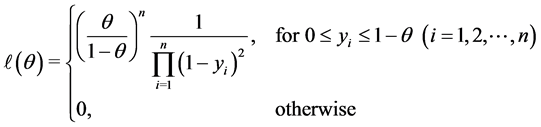
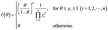
The intermingling of polynomial and logarithmic terms makes method of moments estimation difficult in closed form, as in the SUG case. However, if θ is unknown, the maximum likelihood estimate of θ can be found in a satisfying form, both in the CGUG maximum and CSUG minimum cases. Suppose that  form a random sample from the CSUG Maximum distribution with unknown θ. Since the pdf of each observation has the following form:

the likelihood function is given by
The MLE of θ is a value of θ, where  for
for , which maximizes
 . Let
. Let .
.
Since , it follows that
  is a increasing function, which means the MLE is the largest possible value of θ such that
  for
for . Thus, this value should be
 , i.e.,
 .
.
Suppose next that  form a random sample from the CSUG minimum distribution. Since the pdf of each observation has the following form:

it follows that the likelihood function is given by
As above, it now follows that . It is not too hard to write down the distribution of the MLE’s but we do not do so here.
5. A Summary of Some Other Models
The general scheme given by (3) and (4) is quite powerful. As another example, suppose (using the example from Section 1) that
and . Then it is easy to show that

and that . (The expected value of Y can also be calculated by using the identity
 . In this section, we collect some more results of this type, without proof:
UNIFORM-POISSON MODEL. Here we let  and
and , so that N follows a left-truncated Poisson distribution.
Proposition 5.1. Under the Uniform-Poisson model,


In some sense, the primary motivation of this paper was to produce extreme value distributions that did not fall into the Beta family (such as 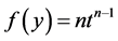 for the maximum of n i.i.d.
  variables). A wide variety of non-Beta-based distributions may be found in [6] . Can we add extreme value distributions to that collection? In what follows, we use both the Beta families
  and
and , the arcsine distribution, and a “Beyond Beta” distribution, the Topp-Leone distribution [15] , as “input variables” to make further progress in this direction.
GEOMETRIC-BETA(2, 2) MODEL. Here  and
and . In this case we get

and

POISSON-BETA(2, 2) MODEL. Here  and
and , the Poisson (q) distribution left- truncated at 0. In this case we get
and
GEOMETRIC-ARCSINE MODEL. Here  and
and . In this case we get

and

POISSON-ARCSINE MODEL. Here  and
and . Here we have

and

GEOMETRIC-TOPP-LEONE MODEL. Here  and
and :
:

and

POISSON-TOPP-LEONE MODEL.  and
and :
:

and

6. Conclusion
In this paper we studied a general scheme for the distribution of the maximum or minimum of a random number of i.i.d. random variables with compact support. While some of the distributions obtained through this process have appeared before in the literature, they do not been studied using this approach. Our biggest open problem is to find data sets for which these new distributions are appropriate.
Acknowledgements
The research of AG was supported by NSF Grants 1004624 and 1040928. We thank the referees for their insightful suggestions for improvement.
Cite this paper
Jie Hao,Anant Godbole, (2016) Distribution of the Maximum and Minimum of a Random Number of Bounded Random Variables. Open Journal of Statistics,06,274-285. doi: 10.4236/ojs.2016.62023
References
- 1. Durrett, R. (1991) Probability: Theory and Examples. Wadsworth and Brooks/Cole, Pacific Grove.
http://dx.doi.org/10.4236/am.2012.34054 - 2. Louzada, F., Roman, M. and Cancho, V. (2011) The Complementary Exponential Geometric Distribution: Model, Properties, and a Comparison with Its Counterpart. Computational Statistics and Data Analysis, 55, 2516-2524.
http://dx.doi.org/10.1016/j.csda.2010.09.030 - 3. Louzada, F., Bereta, E. and Franco, M. (2012) On the Distribution of the Minimum or Maximum of a Random Number of i.i.d. Lifetime Random Variables. Applied Mathematics, 3, 350-353.
- 4. Morais, A. and Barreto-Souza, W. (2011) A Compound Class of Weibull and Power Series Distributions. Computational Statistics and Data Analysis, 55, 1410-1425.
- 5. Johnson, N., Kotz, S. and Balakrishnan, N. (1995) Continuous Univariate Distributions. Vol. 2, Wiley, New York.
- 6. Kotz, S. and van Dorp, J. (2004) Beyond Beta: Other Continuous Families of Distributions with Bounded Support and Applications. World Scientific Publishing Co., Singapore.
http://dx.doi.org/10.1142/5720 - 7. Leadbetter, M., Lindgren, G. and Rootzén, H. (1983) Extremes and Related Properties of Random Sequences and Processes. Springer Verlag, New York.
http://dx.doi.org/10.1007/978-1-4612-5449-2 - 8. Earthquake Data Set.
http://www.data.scec.org/eq-catalogs/date_mag_loc.php - 9. Chung, F., Lu, L. and Vu, V. (2003) Eigenvalues of Random Power Law Graphs. Annals of Combinatorics, 7, 21-33.
http://dx.doi.org/10.1007/s000260300002 - 10. Aiello, B., Chung, F. and Lu, L. (2001) A Random Graph Model for Power Law Graphs. Experimental Mathematics, 10, 53-66.
http://dx.doi.org/10.1080/10586458.2001.10504428 - 11. Marshall, A. and Olkin, I. (1997) A New Method of Adding a Parameter to a Family of Distributions with Applications to the Exponential and Weibull Families. Biometrika, 84, 641-652.
http://dx.doi.org/10.1093/biomet/84.3.641 - 12. Kumaraswamy, P. (1980) A Generalized Probability Density Function for Double-Bounded Random Processes. Journal of Hydrology, 46, 79-88.
http://dx.doi.org/10.1016/0022-1694(80)90036-0 - 13. Urzúa, C.M. (2000) A Simple and Efficient Test for Zipf’s Law. Economics Letters, 66, 257-260.
http://dx.doi.org/10.1016/S0165-1765(99)00215-3 - 14. Aban, I.B., Meerschaert, M.M. and Panorska, A.K. (2006) Parameter Estimation for the Truncated Pareto Distribution. Journal of the American Statistical Association, 101, 270-277.
http://dx.doi.org/10.1198/016214505000000411 - 15. Topp, C.W. and Leone, F.C. (1955) A Family of J-Shaped Frequency Functions. Journal of the American Statistical Association, 50, 209-219.
http://dx.doi.org/10.1080/01621459.1955.10501259