Open Journal of Statistics
Vol.04 No.08(2014), Article ID:49944,8 pages
10.4236/ojs.2014.48057
A Fully Bayesian Sparse Probit Model for Text Categorization
Behrouz Madahian1, Usef Faghihi2
1Department of Mathematical Sciences, University of Memphis, Memphis, TN, USA
2Department of Computing and Technology, Cameron University, Lawton, OK, USA
Email: bmdahian@memphis.edu, ufaghihi@cameron.edu
Copyright © 2014 by authors and Scientific Research Publishing Inc.
This work is licensed under the Creative Commons Attribution International License (CC BY).
http://creativecommons.org/licenses/by/4.0/


Received 22 May 2014; revised 20 June 2014; accepted 18 July 2014
ABSTRACT
Nowadays a common problem when processing data sets with the large number of covariates compared to small sample sizes (fat data sets) is to estimate the parameters associated with each covariate. When the number of covariates far exceeds the number of samples, the parameter estimation becomes very difficult. Researchers in many fields such as text categorization deal with the burden of finding and estimating important covariates without overfitting the model. In this study, we developed a Sparse Probit Bayesian Model (SPBM) based on Gibbs sampling which utilizes double exponentials prior to induce shrinkage and reduce the number of covariates in the model. The method was evaluated using ten domains such as mathematics, the corpuses of which were downloaded from Wikipedia. From the downloaded corpuses, we created the TFIDF matrix corresponding to all domains and divided the whole data set randomly into training and testing groups of size 300. To make the model more robust we performed 50 re-samplings on selection of training and test groups. The model was implemented in R and the Gibbs sampler ran for 60 k iterations and the first 20 k was discarded as burn in. We performed classification on training and test groups by calculating P (yi = 1) and according to [1] [2] the threshold of 0.5 was used as decision rule. Our model’s performance was compared to Support Vector Machines (SVM) using average sensitivity and specificity across 50 runs. The SPBM achieved high classification accuracy and outperformed SVM in almost all domains analyzed.
Keywords:
Bayesian LASSO, Shrinkage, Parameter Estimation, Generalized Linear Models, Machine Learning

1. Introduction
Nowadays, it is usual to come across data sets involving thousands or millions of covariates [3] . A common problem when dealing with fat data sets is that the number of covariates to be estimated far exceeds the number of samples, for instance, text categorization (our focus in this article), gene expression analysis, theft detection, clinical diagnosis, and some business data mining tasks. In text categorization, we need to deal with hundreds even thousands of words in several documents. Given different categories such as mathematics, an attempt to categorize the documents based on their contents (i.e., words) can be cast as a variable selection regression problem with words as covariates in the regression. Furthermore, we need to focus on identifying relevant words to each specific category (i.e., mathematics). That is, predicting the type of documents based on their words composition. However, many covariates may have tiny effects on the category predictions, making it impossible to confidently identify categories based on a single covariate analysis at a time. Thus, a method that can discover the most informative covariates (words) among the large number of covariates (i.e. words related to a specific category in our context) while geared toward highlighting important ones is of a great interest. Many fields are dealing with the problem of identifying important covariates (in our case important words) in a regression model, sometimes known as feature selection [4] [5] .
Depending on the response variable being discrete (categorical) or continuous, different models have been used to perform prediction and estimation: 1) discrete: Logistic Regression (LR) among others have been used to fit models with discrete/categorical response variables. A drawback using logistic LR is that when the number of covariates is large, maximum likelihood estimation becomes computationally intensive and sometimes intractable. Furthermore, predictors may have large estimated variances which result in poor prediction accuracy [1] ; 2) continuous: linear regression models have been extensively used to fit models with continuous response variables. However these models lack accuracy when it comes to parameter estimation in high dimensional data settings [6] . A standard method that is widely used in regression models to improve prediction and parameter estimation is subset selection. Subset selection is a discrete process and has variants such as backward elimination, forward selection, and stepwise selection. However, using these discrete processes may cause inconsistency in variable selection. That is, a small change in the data may result in very different models [4] [6] . In addition, these approaches are computationally expensive and unstable when sample sizes are much smaller than the number of covariates [4] [5] . Given the aforementioned models drawbacks, researchers sought to develop methods that are able to simultaneously analyze multiple covariates [7] -[9] . In the context of text categorization, the response variable or categories (i.e., mathematics) can be binary or multinomial (categorical) for which simple linear regression is not applicable. One alternative to deal with categorical response variables that we have adapted in this paper is using sparse Probit Regression (PR) method. PR is used to link the covariates to the categorical response variable by using cumulative distribution of standard normal distribution [10] . In this paper, we developed a Sparse Probit Bayesian Model (SPBM) to avoid over-fitting problem and obtain fully conditional distributions for all parameters. While shrinking some unimportant covariates to zero SPBM allows us to identify smaller subset of covariates having the greatest discriminating power. To create our model, we first developed a multi-level Bayesian hierarchical model. Then, based on the Gibbs sampling algorithm developed, we used Markov Chain Monte Carlo method to estimate the parameters associated with the covariates [11] [12] . The developed SPBM automatically shrinks small coefficients to zero, which is a great flexibility to fit many covariates to the model in one step. Finally, the fitted model is used to perform classification on different datasets. The rest of this paper will be as follows, in Section 2, we will first briefly describe related works regarding parameter estimation with different methods. We will then explain our method, which includes the construction of a SPBM, MCMC, and using the posterior mean of parameters for prediction. We finally, show our results in the section Application and Results.
2. Related Works
In this section we will make a very brief overview of the machine learning algorithms and other important methods that are used parameter estimation. Support Vector Machines (SVMs) are an alternative that is used in machine learning to deal with high dimensionality and sparsity of data [13] -[15] . Despite small sample sizes, SVMs usually achieve low-test errors. Several papers have reported good results on the applications that use SVMs for variable selections purposes [16] [17] . However, the method has a number of disadvantages, such as the absence of probabilistic output and the necessity of estimating a trade-off parameter in order to utilize Mercer kernel functions [4] [5] . David Blei et al. [18] using Latent Dirichlet Allocation (LDA) [19] , introduced a machine learning algorithm to Probabilistic Topic Modeling (PTM). PTM aims at automatically extracting topics from texts. That is, for instance, if we apply the algorithm to the last few discourse of a politician, it produces economy, war, jobs as the output. The relevance of the probabilistic modeling to our paper is that the algorithm extracts the topics. Thus, in some cases, it is possible to consider the most rated topic in a text as the topic of the text. However, LDA performance is compared by some researchers as nothing more than the iterative keyboard searching algorithms [20] . The algorithm is also limited to the words used in the text. For instance, if you are looking for consciousness, and give a text regarding civil engineering to the algorithm as input, the algorithm will only tell you about building and constructions [21] .
Another method that is used in statistics for parameter estimation is linear regression. It is an approach to model the relationships between the response variables and one or several covariates. The method has been extensively used in different applications. In linear regression models, Ordinary Least Square (OLS) method is used to obtain the estimation of the parameters. OLS estimates parameters by minimizing sum of residual squared error. However, the method suffers from two drawbacks: 1) even though the estimated parameters obtained by the model have low bias, they often have large variance that reduces the accuracy of the prediction by the model; 2) when there are large number of covariates, it is desirable to establish a small subset of parameters which offers the strongest effect on response variable [6] . In OLS, estimation accuracy can be improved by setting the unimportant covariates to zero and thus obtaining more accurate estimates for significant covariates [6] . We will discuss the know how about this method in our method section.
Logistic regression is a generalized linear model approach, which is used for modeling when the response variable is categorical. In text categorization, logistic regression methods are commonly used to find maximum likelihood estimations of parameters that are associated with covariates. For instance, many software packages use a variation of Newton-Raphson’s iterative algorithm [22] or Fisher’s scoring method [23] . To find maximum likelihood estimates, the aforementioned packages, implement maximization procedures, which use matrix inversion. However, when the numbers of covariates are very large, matrix inversion method is computationally intensive. Thus, the estimated results often suffer from poor accuracy and lack of convergence to the true value of parameters that are associated with covariates-which is global maxima [1] . Furthermore, these methods fail when the number of parameters to be predicted far exceeds the number of observations. As a result, the above methods cannot perform parameter estimation and good classification when it comes to large number of covariates [4] . Thus, for text categorization to analyze data sets with sample sizes that are much smaller than the number of covariates, new methods are required. One alternative to avoid overfitting is highly regularized approaches such as penalized regression models. These models are needed to identify non-zero coefficients, enhance model predictability and avoid over-fitting [5] [24] . A widely used model to avoid overfitting problem is the shrinkage and regularization method which can improve parameter estimation performance by reducing mean square error while introducing some bias [6] [25] . Furthermore, by inducing sparseness in the model, shrinkage method highlights important covariates. Such methods facilitate the analysis of many covariates simultaneously [7] . To avoid overfitting problem in text categorization, authors in [2] , used a Bayesian approach to logistic regression. They used a prior probability distribution that favors sparseness in the model, and an optimization algorithm that is geared toward finding maximum a posteriori as point estimates of parameters. However, their optimization method is a local optimization, which results in point estimate of parameters. Accordingly, the method does not provide full posterior distributions of parameters.
Among others, Least Absolute Shrinkage and Selection Operator (LASSO), is one of the very efficient penalized regression method that is widely used for the model fitting purpose and the prediction of response variables [2] [6] [26] -[30] . A Bayesian LASSO method was proposed by [31] [32] in which double exponential prior is used on parameters in order to impose sparsity in the model. To allow data adaptive prior choice, LASSO can also be extended by expressing double exponential distributions as a scale mixture of normal distributions [31] - [33] . In this paper, we considered a Sparse Probit Bayesian Model by assigning double exponential prior distribution to parameters that favor sparseness in terms of the number of used variables. Furthermore, the fully Bayesian approach adopted here provides us with posterior distributions of parameters which can be used for different prediction (classification) and estimation purposes.
3. Methods
In order to set up the model, we first obtain the fully conditional distributions for all parameters in a multi-level hierarchical model. In the second step, the Markov Chain Monte Carlo (MCMC) method based on Gibbs sampling algorithm developed is used to estimate all the parameters [11] [12] . The sparse multi-level Bayesian hierarchical model is implemented to control the issue of over-fitting that arises when too many variables are included in the model. The SPBM automatically shrinks small coefficients to zero. Thus, the model shows a great flexibility to fit many covariates at the same time. In step three, we will use the fitted model to perform classification on different datasets. As it mentioned above, since the response variables are categorical, prior to develop the fully Bayesian model, some treatment of the response variables are required: Let  represent the observed response variables-assuming the documents are from two categories “a” and “b”. Suppose
  if the category is “a” and 0 otherwise. Let
  represent the weight associated with word j in document i. Since, the response variables are discrete the error term does not satisfy the normality of error variance assumption which is required in order to fit linear regression models. Furthermore, simple linear regression model if used may not produce legitimate results. In the context of Generalized Linear Models (GLM), nonlinear link functions have been used in order to associate the nonlinear and discrete response variable y to the linear predictor
 .
.  is a
is a  vector, representing weights of the words one to word p in document i, and p is the number of words used in the model.
  is the
  vector of model parameters (in our case associated with word to word). Let H represent the link function between nonlinear and discrete response variable y and the linear predictor
 . The GLM model can be represented as (Formula (1)):
 (1)
(1)
In this formula,  is the covariates vector for document i. Following [34] , we use Probit link function (Formula (2)) which corresponds to Probit regression model and is applicable to binary and multi-level outcome (response variables) situations.
 (2)
(2)
In this formula Φ−1 is the inverse of cumulative distribution function of standard normal distribution. In order to be able to find the posterior distributions of parameters, we need to integrate the likelihood function multiplied by joint prior distributions of all parameters. However, the model with the current configuration makes the integration intractable. Thus, following [34] , “n” independent latent variables  with
with  are introduced to the model and the following relationship between response variable and its corresponding latent variable is established. This way the Probit regression model for binary outcome
  is linked to the linear regression model for the latent variable
  (Formula (3)).
 (3)
(3)
In the following, we explain how we implemented a fully Bayesian hierarchical model and prior distributions. In the continuation of step one, in order to set up a fully Bayesian hierarchical model, we will use an independent double exponential prior distributions on  as follows (Formula (4)).
 (4)
(4)
In the above formula,  is the hyper-parameters of the distribution which can be selected or assigned to a distribution and predicted with other parameters. In our analysis, following Bae and Mallick [35] , we set
  so that
 . Double exponential distribution (left side of Formula (5)) can be represented as scale mixture of normal with an exponential mixing density (Formula (5)) [31] [35] .
 (5)
(5)
This hierarchical representation will be used in order to be able to set up the Gibbs sampling algorithm. Having , the following hierarchical prior distribution is used to set up the Gibbs sampler:
 ;
; , with
  if
if . Using the above mixture representa-
tion for the parameters and defined prior distributions, we obtain the fully conditional posteriors that lead to a straightforward Gibbs sampling algorithm.
 (6)
(6)
In Formula (6), TN stands for truncated normal distribution and  represents vector of model parameters plus data. For observation “i” with
 ,
,  must be sampled from the normal distribution defined truncated above zero or below zero if
 .
.

In Formula (7), fully conditional posterior distribution of vector of model parameters is multivariate normal distribution (MVN) with mean vector and variance covariance matrix as specified where . In (7), X is the
  design matrix in which
  represents weight of word j in ith sample (document) and p is the number of words (covariates) in the model and
  and “n” is the number of samples. The fully conditional distribution of hyper-parameters
 ,
,  , are inverse-Gaussian distribution with loca-
tion  and scale
 . In each iteration of the Gibbs sampling,
  is sampled from the inverse Gaussian distribution defined in Equation (8).

4. Data Preparation
In this step, we move forward to process documents based on their word composition. To do so, assuming that we have samples from different types of documents, we process each document’s content based on the document composition. Among different methods that are used to represent documents for statistical classification, we chose term weighting [2] . To do so, for each unique term in texts, we first created a term-document matrix. Then, for each unique word in the matrix, we calculated the frequency of the words in each document—how important is the word in the document. We also computed the importance of the word in all documents. To calculate the weight of each term in all documents, we used a type of TF*IDF (term frequency times inverse document frequency) term weighting with cosine normalization [2] . In this method each term (word) j in document i has a un-normalized primitive weight of:
 (9)
(9)
In the above formula  is the number of times that term j occurs in document i.
  is the number of documents in which term j exists.
  is the total number of documents. Then to minimize the impact of the document length, we cosine-normalize the feature vectors to have a Euclidian norm of 1.0.

5. Application and Results
Ten domains including, Mathematics, Chemistry, Computer Science, Psychology, Neuroscience, Art, Physics, Electronic, Biology, and Geology are explored in this study. We first downloaded the entire domains corpus from Wikipedia which included 60 documents for each domain. We then, created the TFIDF matrix and then for each domain divided the whole data set randomly into training and testing data sets of the same size. Each domain’s training and test documents were randomly divided into 300 separate documents having each more than 3000 words as follows. For each domain, 30 documents out of 60 is chosen randomly as those with  to be a part of training and test data sets and the remaining documents (540)
  is randomly divided in two. Thus, we ended up with 300 training samples and 300 test samples. This approach was adopted, to ensure that training and test samples both contain the documents with
 . In order to make the model more robust we performed 50 re-samplings on selection of training and test groups and re-ran the model. The model was implemented in R and the Gibbs sampler ran for 60 k iterations and the first 20 k is discarded as burn in. We performed classification on training data set and test datasets by calculating
  and using the threshold of 0.5 for decision rule [2] . This threshold has been used in research papers for the purpose of classification [2] [36] . In our model, binary classifier is defined as the document belonging to the domain or not. There are almost 18,000 unique words in the whole corpus. Without loss of generality, we performed two-sample t-test on the TFIDF matrix in order to rank words based on their differences in distribution between all domains documents. The top 800 words that obtained from this procedure were used as input to the model. For each domain, we trained the model and posterior mean of θs were used for covariate selection and classification. Using top 80 words based on absolute value of posterior mean of θs the obtained classifier for each domain predicted the probability of whether a document belongs to the category. Figure 1 represents the posterior mean of θs associated with words. While some noise like signals—words that do not have distinguishing power—are shrunk toward zero, other signals stand out, which turn out to be more relevant to the document classifiers.
As explained above, we used top 80 words obtained from the moel for the purpose of classification on train and test groups. Table 1 and Table 2 represent the result of classification for training and testing phases. For instance, the probability of a document belonging to mathematics  is calculates as
  and
and . In which
  is cumulative distribution function of standard normal distribution
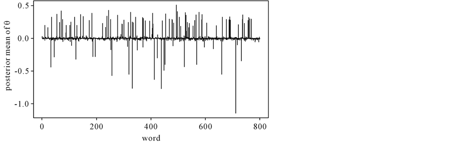
Figure 1. Posterior mean of θ.

Table 1. Average sensitivity and specificity of the SPBM compared to SVM for training groups.
Table 2. Average sensitivity and specificity of the SPBM compared to SVM for test groups.
and  the vector representing weights of the selected words for classification in document i.
  is the associated posterior means of model parameters. In order to assess the classification accuracy of the model, we used sensitivity and specificity measures. Sensitivity and specificity are statistical measures that evaluate performance of binary classifiers [37] . Sensitivity measures the proportion of actual positives (i.e., math documents) that are identified by the model to be positive (i.e., math) and specificity measures the proportion of negatives (i.e. non-math docs) that are correctly classified as negative (non-math). In order to compare our results to SVM, we used the same procedure in dividing the data into train and test groups and performed 50 re-sampling and recorded the average sensitivity and specificity across 50 runs. In order to perform SVM analysis, we used Kernlab [38] [39] library in R. The average Sensitivity and specificity results for training and test groups using our model and SVM are shown in Table 1 and Table 2. Based on Table 2 results, in eight out of ten categories for test groups, on average the sensitivity and specificity of SPBM outperforms SVM. Table 2 also shows that, in Art and physics domains the specificity of SVM is better than SPBM and in terms of the sensitivity of SVM outperforms SPBM in computer science and chemistry domains. However, the results obtained from SPBM on these categories are very comparable to SVM. As we can see, the overall results suggest that SPBM outperforms SVM in classification.
6. Conclusion
Covariates selection and parameter estimation are the main issues that researchers dealing with datasets with the large number of covariates with small sample sizes need to overcome. Therefore, highly regularized approaches, such as penalized regression models, are needed to identify non-zero coefficients, enhance model predictability and avoid overfitting [6] [40] . In addition, continuous response variables which are a requirement of linear regression methods are not applicable to response variables (phenotypes) that are dichotomous. To address these limitations, we developed a Sparse Probit Bayesian Model by imposing double exponential prior on parameters and evaluated its performance using 10 different corpuses. To obtain posterior distribution of covariates based on the Gibbs algorithm developed, we used a Markov Chain Monte Carlo based technique. Based on Table 2 results, in eight out of ten categories for test groups, on average the sensitivity and specificity of SPBM outperform SVM. Table 2 also shows that, in art and physics domains the specificity of SVM is slightly better than SPBM and in terms of the sensitivity of SVM outperforms SPBM in computer science and chemistry domains. However, the results obtained from SPBM on these categories are very comparable to SVM. Taken all together these results suggest that SPBM outperforms SVM in classification. Furthermore, in this paper, we have developed a model that enabled us to, from a big corpus, distinguish a small number of words having the greatest discriminating power. We used top 80 covariates obtained for the purpose of classification and the probability of each sample belonging to one of the categories of outcome was calculated. Additionally, the model achieved high classification accuracy for categorizing texts (Table 1 and Table 2). Taken together our results suggest that the SPBM applied to 10 different corpuses downloaded from Wikipedia allows for better class prediction and produces higher classification sensitivity and specificity. Our future plan is to evaluate the model performance while considering more complex variance-covariance matrix structure, which takes into account word-word interactions (correlations). Also, future work will investigate using different link functions and their effects on the model performance. Lastly, we plan to extend the model to other sparse models, which use specialized prior distributions with heavier tails that might offer more robustness properties.
References
- Pike, M., et al. (1980) Bias and Efficiency in Logistic Analyses of Stratified Case-Control Studies. International Journal of Epidemiology, 9, 89-95. http://dx.doi.org/10.1093/ije/9.1.89
- Genkin, A., Lewis, D.D. and Madigan, D. (2007) Large-Scale Bayesian Logistic Regression for Text Categorization. Technometrics, 49, 291-304. http://dx.doi.org/10.1198/004017007000000245
- Cao, J. and Zhang, S. (2010) Measuring Statistical Significance for Full Bayesian Methods in Microarray Analyses. Bayesian Analysis, 5, 413-427. http://dx.doi.org/10.1214/10-BA608
- Li, J., et al. (2011) The Bayesian Lasso for Genome-Wide Association Studies. Bioinformatics, 27, 516-523. http://dx.doi.org/10.1093/bioinformatics/btq688
- Bae, K. and Mallick, B.K. (2004) Gene Selection Using a Two-Level Hierarchical Bayesian Model. Bioinformatics, 20, 3423-3430. http://dx.doi.org/10.1093/bioinformatics/bth419
- Tibshirani, R. (1996) Regression Shrinkage and Selection via the Lasso. Journal of the Royal Statistical Society Series B, 58, 267-288.
- Madahian, B., Deng, L.Y. and Homayouni, R. (2014) Application of Sparse Bayesian Generalized Linear Model to Gene Expression Data for Classification of Prostate Cancer Subtypes. Open Journal of Statistics, 4, 518-526. http://dx.doi.org/10.4236/ojs.2014.47049
- Wu, T.T., et al. (2009) Genome-Wide Association Analysis by Lasso Penalized Logistic Regression. Bioinformatics, 25, 714-721. http://dx.doi.org/10.1093/bioinformatics/btp041
- Yang, J., et al. (2010) Common SNPs Explain a Large Proportion of the Heritability for Human Height. Nature Reviews Genetics, 42, 565-569. http://dx.doi.org/10.1038/ng.608
- Madsen, H. and Thyregod, P. (2011) Introduction to General and Generalized Linear Models. Chapman & Hall/CRC, Boca Raton.
- Gelfand, A. and Smith, A.F.M. (1990) Sampling-Based Approaches to Calculating Marginal Densities. Journal of the American Statistical Association, 85, 398-409. http://dx.doi.org/10.1080/01621459.1990.10476213
- Gilks, W.R., Richardson, S. and Spiegelhalter, D. (1995) Markov Chain Monte Carlo in Practice. Chapman and Hall/CRC, London.
- Leopold, E. and Kindermann, J. (2002) Text Categorization with Support Vector Machines. How to Represent Texts in InPut Space? Machine Learning, 46, 423-444. http://dx.doi.org/10.1023/A:1012491419635
- Kim, H., Howland, P. and Park, H. (2005) Dimension Reduction in Text Classification with Support Vector Machines. Journal of Machine Learning Research, 6, 37-53.
- Joachims, T. (1998) Text Categorization with Support Vector Machines: Learning with Many Relevant Features. Springer, Berlin Heidelberg.
- Guyon, I., et al. (2002) Gene Selection for Cancer Classification Using Support Vector Machines. Machine Learning, 46, 389-422. http://dx.doi.org/10.1023/A:1012487302797
- Weston, J., et al. (2002) Feature Selection for SVMs. Advances in Neural Information Processing Systems. MIT Press, Cambridge.
- Blei, D.M. (2012) Probabilistic Topic Models. Communications of the ACM, 55, 77-84. http://dx.doi.org/10.1145/2133806.2133826
- Blei, D.M., Ng, A.Y. and Jordan, M.I. (2003) Latent Dirichlet Allocation. The Journal of Machine Learning Research, 3, 993-1022.
- Schmidt, B. (2013) Sapping Attention: Keeping the Words in Topic Models. http://sappingattention.blogspot.com/2013/01/keeping-words-in-topic-models.html
- Weingart, S.B. (2012) Topic Modeling for Humanists: A Guided Tour. http://www.scottbot.net/HIAL/?p=19113
- Wedderburn, R.W.M. (1974) Quasi-Likelihood Functions, Generalized Linear Models, and the Gauss-Newton Method. Biometrika, 61, 439-447.
- Jennrich, R.I. and Sampson, P.F. (1976) Newton-Raphson and Related Algorithms for Maximum Likelihood Variance Component Estimation. Technometrics, 18, 11-17. http://dx.doi.org/10.2307/1267911
- Hastie, T., Tibshirani, R. and Friedman, J. (2009) Linear Methods for Regression. Springer, New York.
- Hoerl, A.E. and Kennard, R.W. (1970) Ridge Regression: Biased Estimation for Nonorthogonal Problems. Technometrics, 12, 55-67. http://dx.doi.org/10.1080/00401706.1970.10488634
- Li, Z. and Sillanpää, M.J. (2012) Overview of LASSO-Related Penalized Regression Methods for Quantitative Trait Mapping and Genomic Selection. Theoretical and Applied Genetics, 125, 419-435. http://dx.doi.org/10.1007/s00122-012-1892-9
- Knight, K. and Fu, W. (2000) Asymptotics for Lasso-Type Estimators. The Annals of Statistics, 28, 1356-1378. http://dx.doi.org/10.1214/aos/1015957397
- Yuan, M. and Lin, Y. (2005) Efficient Empirical Bayes Variable Selection and Estimation in Linear Models. Journal of the American Statistical Association, 100, 1215-1225. http://dx.doi.org/10.1198/016214505000000367
- Zou, H. (2006) The Adaptive Lasso and Its Oracle Properties. Journal of the American Statistical Association, 101, 1418- 1429. http://dx.doi.org/10.1198/016214506000000735
- Zou, H. and Li, R. (2008) One-Step Sparse Estimates in Non-Concave Penalized Likelihood Models. The Annals of Statistics, 36, 1509-1533. http://dx.doi.org/10.1214/009053607000000802
- Park, T. and Casella, G. (2008) The Bayesian Lasso. Journal of the American Statistical Association, 103, 681-686. http://dx.doi.org/10.1198/016214508000000337
- Hans, C. (2009) Bayesian Lasso Regression. Biometrika, 96, 835-845. http://dx.doi.org/10.1093/biomet/asp047
- Griffin, J.E. and Brown,P.J. (2007) Bayesian Adaptive Lassos with Non-Convex Penalization. Technical Report, IMSAS, University of Kent, Canterbury.
- Albert, J. and Chib, S. (1993) Bayesian Analysis of Binary and Polychotomous Response Data. Journal of the American Statistical Association, 88, 669-679. http://dx.doi.org/10.1080/01621459.1993.10476321
- Bae, K. and Mallick, B.K. (2004) Gene Selection Using a Two-Level Hierarchical Bayesian Model. Bioinformatics, 20, 3423-3430. http://dx.doi.org/10.1093/bioinformatics/bth419
- Chen, J., et al. (2006) Decision Threshold Adjustment in Class Prediction. SAR and QSAR in Environmental Research, 17, 337-352. http://dx.doi.org/10.1080/10659360600787700
- Altman, D.G. and Bland, J.M. (1994) Diagnostic Tests 1: Sensitivity and Specificity. British Medical Journal, 308, 1552. http://dx.doi.org/10.1136/bmj.308.6943.1552
- Karatzoglou, A., Meyer, D. and Hornik, K. (2005) Support Vector Machines in R. Journal of Statistical Software, 15, 1-28.
- Karatzoglou, A., et al. (2004) Kernlab—An S4 Package for Kernel Methods in R. Journal of Statistical Software, 11, 1-20.
- Williams, P.M. (1995) Bayesian Regularization and Pruning Using a Laplace Prior. Neural Computation, 7, 117-143. http://dx.doi.org/10.1162/neco.1995.7.1.117