Open Journal of Statistics
Vol.3 No.4(2013), Article ID:35934,7 pages DOI:10.4236/ojs.2013.34030
Change-Point Detection for General Nonparametric Regression Models
Department of Mathematics and Statistics, University of Calgary, Calgary, Canada
Email: *burke@math.ucalgary.ca
Copyright © 2013 Murray D. Burke, Gildas Bewa. This is an open access article distributed under the Creative Commons Attribution License, which permits unrestricted use, distribution, and reproduction in any medium, provided the original work is properly cited.
Received May 1, 2013; revised June 15, 2013; accepted June 22, 2013
Keywords: Change-point detection; Nonparametric regression models; Weighted bootstrap
ABSTRACT
A number of statistical tests are proposed for the purpose of change-point detection in a general nonparametric regression model under mild conditions. New proofs are given to prove the weak convergence of the underlying processes which assume remove the stringent condition of bounded total variation of the regression function and need only second moments. Since many quantities, such as the regression function, the distribution of the covariates and the distribution of the errors, are unspecified, the results are not distribution-free. A weighted bootstrap approach is proposed to approximate the limiting distributions. Results of a simulation study for this paper show good performance for moderate samples sizes.
1. Introduction
Model building is a very important task. When considering observations  taken over time we may wish to consider the relationship between the Xi and the Yi by some regression model, either parametric or semiparametric, linear or nonlinear. However, if, after some point i = k, there is a change in the relationship between Xi and Yi, then a single regression model will be inappropriate and would fit the data poorly. For example, in Figure 1 below, the scatterplot on the left is that of a combined sample of 150 points. The middle scatterplot is that of the first 60 points while the right plot is that of the remaining 90 points. Without realizing that there was a change-point, one might wrongly propose a single regression model, perhaps linear, with heteroscedastic errors. Thus, it is important to determine whether such a change has occurred before the particular form of the model is postulated. If such a change has occurred, then two regression models should be used, one for the first k pairs and another for the remaining pairs. We will propose a number of tests designed to detect whether a change has occurred in a general nonparametric model. Change-point problems arise in many areas when observations (Xi, Yi) are taken over time i.
For example, the height of (or discharge from) a river as a function of upstream precipitation, or concentrations of heavy metals in storm-water runoff as a function of suspended sediment size. We refer to the book by Csörgő and Horváth [1] for more applications and important references and to the papers [2-4] for other change-point problems.
We say that the pair (X, Y) satisfies general regression model M(ϕ, ψ, F, ε) if
for all , where ε is a mean zero, variance one random variable, independent of X. We write (X, Y)
  M(ϕ, ψ, F, ε).
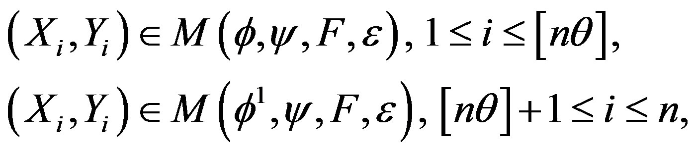
For a sequence , consider the null hypotheses:
 (1)
(1)
where ϕ, ψ > 0, and F are unspecified, the Xi are independent and the εi are independent and identically distributed. Model (1) encompasses both linear and nonlinear regression models and the case of heteroscedastic errors. We wish to test whether there is a change in the model as the observations are taken, without specifying ϕ, ψ or F, that is to test the null Hypothesis (1) versus the alternative:
 (2)
(2)
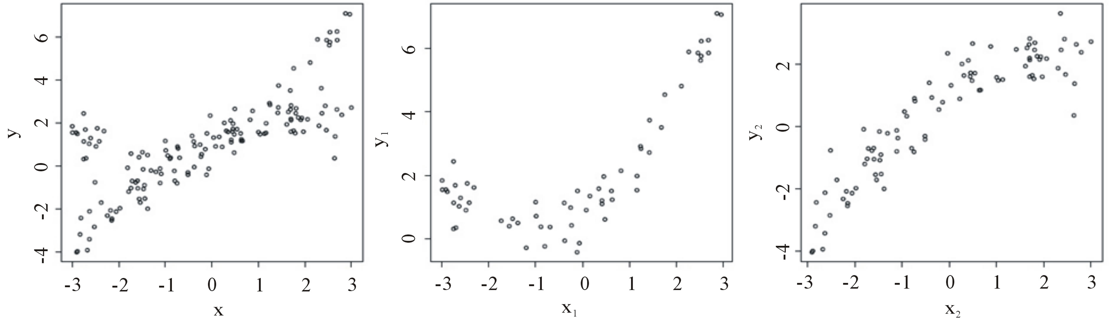
Figure 1. Scatterplot of (Xi, Yi).
for some , where [s] denotes the integer part of s.
 (3)
(3)
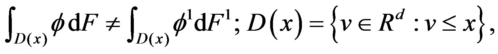
for some , using the usual partial order in
 .
.
The alternative Hypothesis (2) includes the case where only ϕ changes, that is,  , for some
 , and when only F changes
 , for some
 .
.
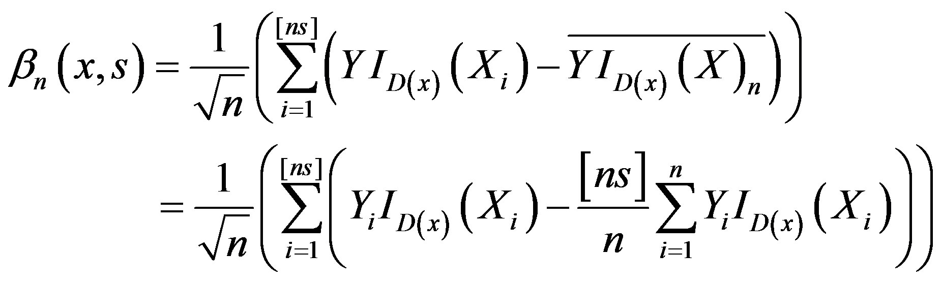
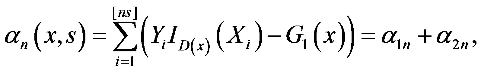
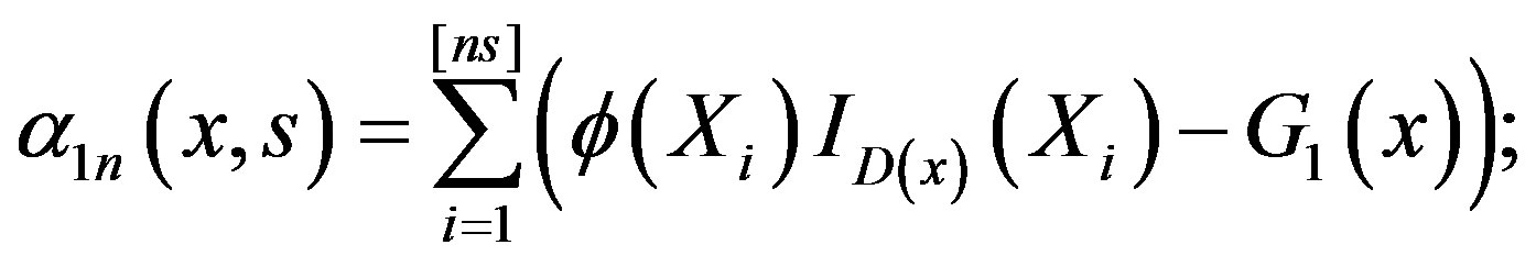
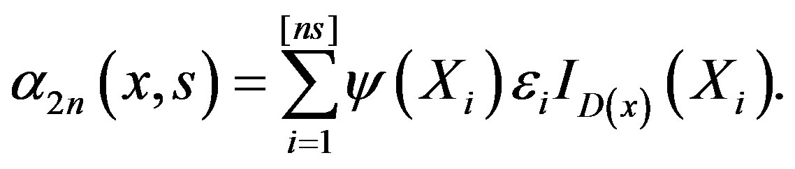
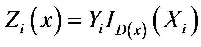
We will base our tests on the process
 and zero otherwise, where
  is the indicator of the event
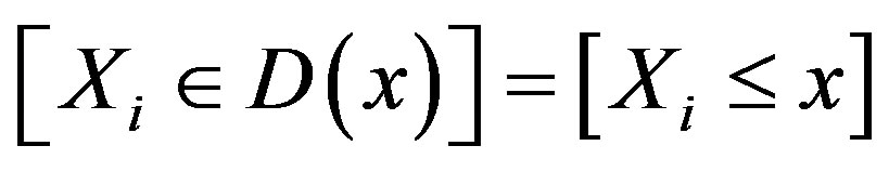
and
 .
.
βn can also be written as the difference of two means
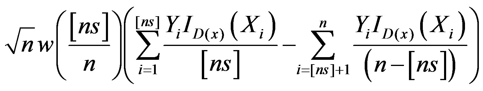 (4)
(4)
where
 .
.
Note that
 .
.
We are considering the partial sums of the response variables Yi aligned according to the Xi-observations. The advantage of βn is that we can use empirical process theory which has much better convergence properties, rather than trying to estimate the function ϕ directly with kernel or other curve estimation methods which require a large sample size. As will be demonstrated in the simulation study, our approach works well for moderate sample sizes.
In the next section, we state the main results related to the weak convergence of the above process as well as convergence of various related statistics. These results do not assume the stringent condition of bounded variation for the regression function ϕ and the variance function ψ and strong moment conditions on the error distribution, which were assumed in an earlier paper [5]. Section 3 states the asymptotic results for the weighted bootstrap version of our statistics. This is needed since the asymptotic distributions of our statistics depend on unspecified functions. A new simulation study is conducted in Section 4. Proofs of the results (different from those in [5,6]) are sketched in Section 5.
2. Main Results
Assume the following:
(A1) The sequences {Xi} and {εi},  are independent.
(A2) The {Xi} are independent and identically distributed random vectors with distribution function F.
(A3) The functions , with
 , satisfy
 .
.
(A4) The {εi: 1 < i} are independent and identically distributed with E({εi) = 0 and .
.
(A5)
 .
.
Conditions (A1)-(A5) are much weaker than those in [5] and [6] where ϕ and ψ needed to be of bounded total variation and εi required much higher moment conditions ( ). While the conclusions in [5] and [6] may be stronger (weighted approximations), the requirement of bounded variation for ϕ and ψ limits their applicability. Here we dispense with this requirement. For example, we permit the case where the Xi have unbounded support and the regression relationship is polynomial (unbounded), provided Xi has finite moments of a suitable degree.
For
 let
let
 .
.
The first main result is:
Theorem 1 Under Assumptions (A1)-(A5) and the null Hypothesis (1),
in the space , equipped with the uniform norm, where
  is mean-zero Gaussian process with covariance function
and where
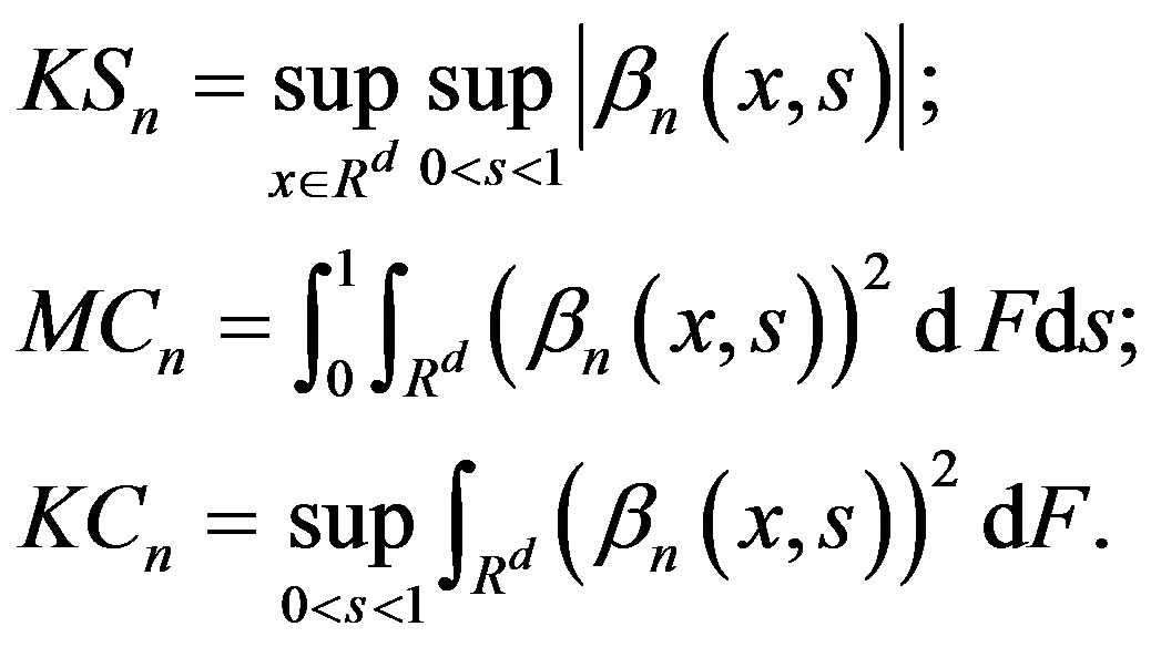
Corollary 2 Under the conditions of Theorem 1 and the null Hypothesis (1),
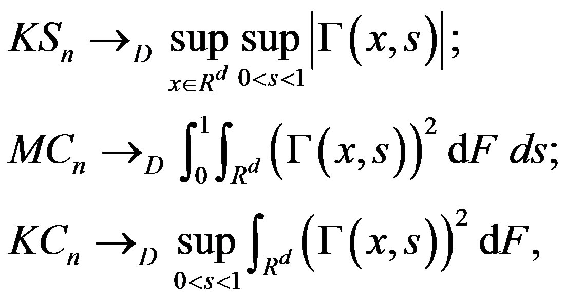 (5)
(5)
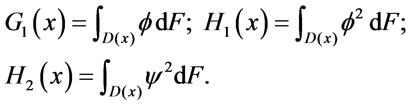
where
 (6)
(6)
Corollary 2 follows immediately from Theorem 1.
Corollary 3 Under Assumptions (A1)-(A5) and (A3) for ϕ1 and F1, the test statistics defined by (6) are consistent against the alternative Hypothesis (2).
Under the null Hypothesis (1),  has mean zero for all x and s. The statistic
  in Equation (6) is a Kolmogorov-Smirnov type statistic expressing the largest deviation between the two means (before [ns] and after [ns]). Both statistics
  and
and  are Cramérvon Mises type statistics which measures the squaredintegral distance between the two means. The statistic
  is the mean (integral over s) such distance, while
  is the supremum of the squared-integral distance.
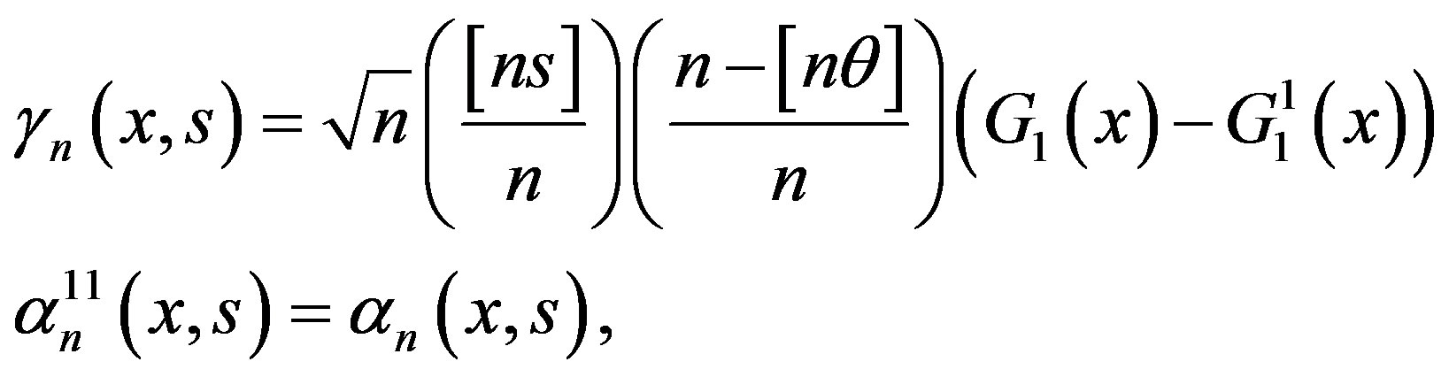
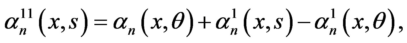
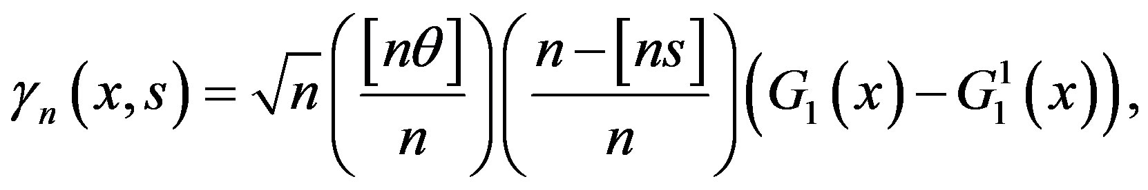
Under the alternative Hypothesis (2), when s < θ, the first part of Expression (4) has mean
 while the term after the minus sign has mean
 when s > θ. (see inequality (3)).
3. Weighted Bootstrap Approximations
Since the distribution functions of the Xi and εi, as well as the functional forms of ϕ and ψ, are not specified, the limiting distributions of all our test statistics will not be known. A weighted bootstrap is proposed here which will approximate these asymptotic distributions.
Let
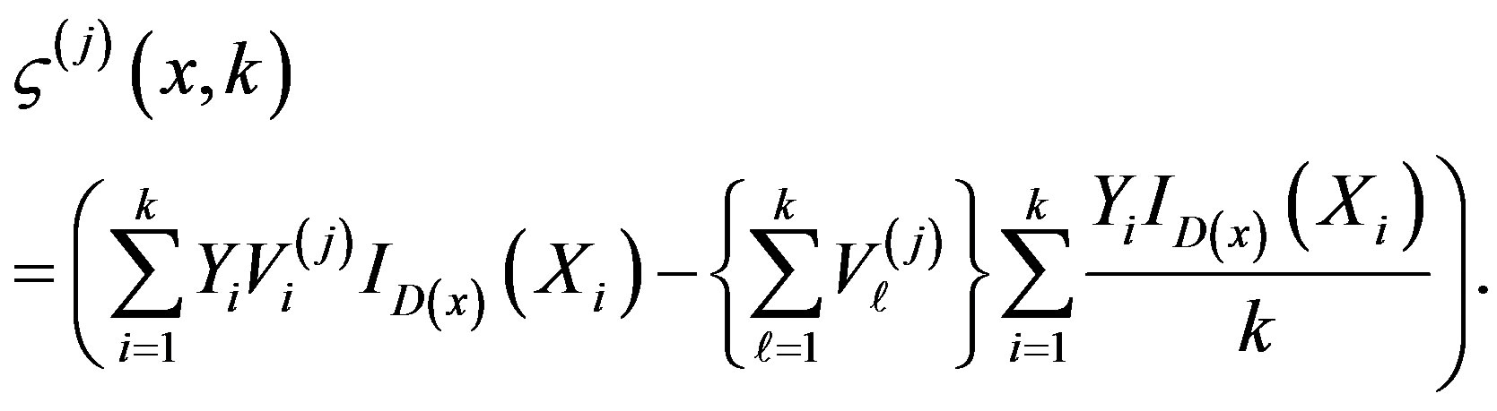
be m independent sequences of independent and identically distributed random variables, independent of the {εi} and {Xi} sequences. We will consider the processes
for
 zero otherwise, where
 , and
, and
Theorem 4 Assume Conditions (A1)-(A5) hold and that (A4)-(A5) holds for the sequences also. Then, under the null Hypothesis (1), along almost all sequences
 given (Xi,Yi),
  ,
,  in the space
 , equipped with the uniform norm, for each j, where
 is a mean-zero Gaussian process.
Under the conditions of Theorem 4, the same limiting distributions as found in Corollary 2 for statistics based on βn are obtained for each . Moreover, the statistics based on βn and
 ,
,  , are asymptotically independent.
It is also important for the bootstrap process to have a limiting distribution under the alternative hypothesis. We obtain:
Theorem 5 If the conditions of Theorem 4 hold for the functions ϕ1, F1 , then under the alternative Hypothesis (2), along almost all sequences , given (Xi,Yi),
  ,
,  in the space
 , equipped with the uniform norm, for each j, where
  is a mean-zero Gaussian process.
4. Simulations
The proposed tests are omnibus tests in that we do not specify the form of the regression function ϕ. In order to examine how these tests perform, we conducted simulations for two quite different functions, ϕ(x) = 1 + x + βx2 and ϕ(x) = 2 sin(βx). The Xi were generated from the uniform U(−3, 3) distribution and the errors εi were standard normals. In each case, 1000 simulations were carried out, each with m = 1000 weighted bootstrap samples. The level of the tests was α = 0.05 throughout. Theorem 3 allows us to choose any mean-zero, variance-one distribution for the bootstrap weights . We chose standard normal weights for the simulation since the limiting processes are Gaussian and normal bootstrap weights have been found to work well in simulations for goodness-of-fit types of statistics [7,8]. We use the percentile method. If h(βn) is one of the statistics in Corollary 2, we reject the null hypothesis if
 , where cn(α) is the (1 − α)100-th percentile of the values
 ,
, . Under the null hypothesis, cn(α)→ c(α), where c(α) is the (1 − α)100-th percentile of
  (Theorems 1 and 3). Under the alternative hypothesis, cn(α)→ c11(α), with c11(α), the (1 − α)100-th percentile of
  and h(βn) →P∞ (Corollary 3 and Theorem 4).
The first power study is for the alternative:
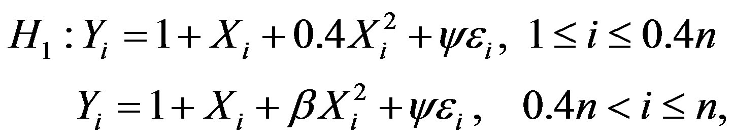
where ψ does not depend on Xi and the change-point is at 0.4n. The statistics KSn, KCn and MCn are defined by Equation (6).
The first three rows correspond to the empirical level of the tests under the null hypothesis (β = 0.4) with different choices for ψ, the standard deviation. The breakpoint θ equals 0.4. The empirical level results are reasonably good especially when n > 50, that is they are close to the level of 0.05. The empirical powers of the tests are in the subsequent rows for different β.
As can be seen in Table 1, the power increases as β gets farther from 0.4 (the null Hypothesis). Understandably the power increases in n and decreases in ψ gets larger.
In the second simulation (see Table 2), we consider ϕ to be a sine function. We conduct our simulations for sample sizes n = 50, 100, 150. The first row of Table 2 is the empirical level of the test (β = 1, no change-point). Again the empirical level is good when n > 50.
We take ψ = 1, but vary the location of the changepoint θn. The power increases as β gets farther from 1 (the null hypothesis). The power increases with the sample size n. Except in a few instances, the power is greatest when the change-point occurs in the middle (θ = 0.5) and decreases as θ is farther from 0.5. The exceptional cases are likely due to simulation error.
Considering that our tests are omnibus in nature, the power results can be seen to be quite good.
5. Proofs of the Main Results
Proof of Theorem 1: For , let
, let
where
The collection is a Vapnik-Cervonenkis class of sets. Consequently, the collection of indicator functions

is a Donsker class of functions. For (fixed) ϕ and ψ,
and
are Donsker classes (Pollard [9]). By Giné and Zinn [10, 11] (see also Corollary 2.9.3 of [12]),
where
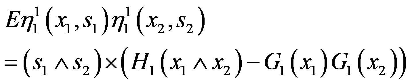
 converges in distribution to a vector of tight independent Gaussian processes, η1
and η2, each with zero mean and covariance (j = 1, 2):

Consequently,
converges in distribution to a vector of tight independent Gaussian processes  with
with  and covariance
 .
.
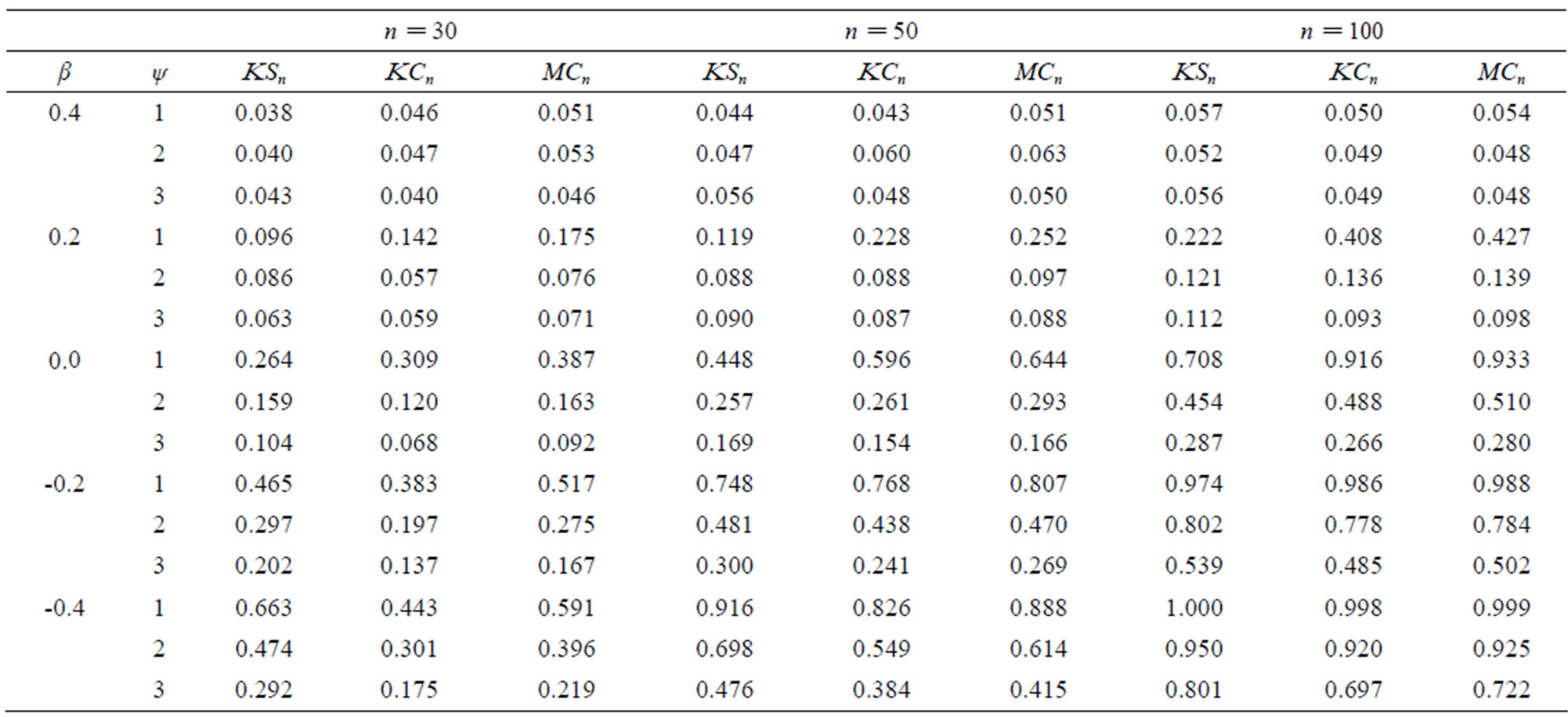
Table 1. Power when ϕ(x) = 1 + x + 0.4x2, ϕ1(x) = 1 + x + ψx2 and breakpoint θ = 0.4.
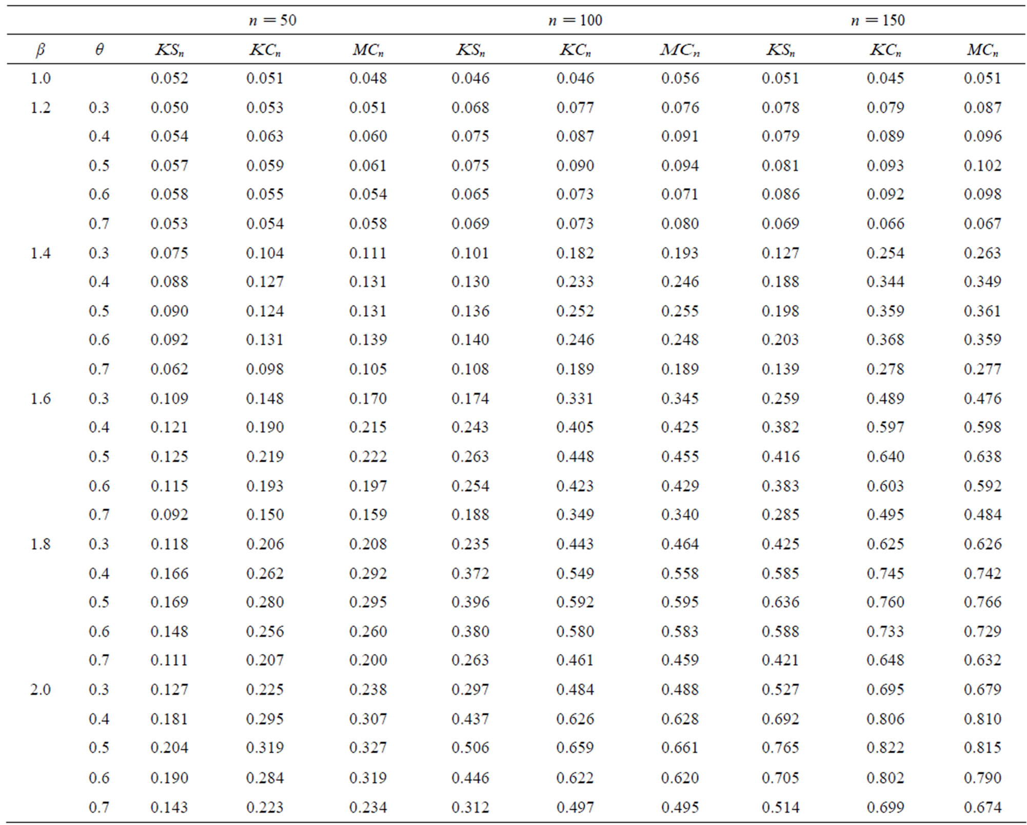
Table 2. Power when ϕ(x) = 2 sin(x), ϕ1(x) = 2 sin(βx), and ψ = 1 with different breakpoints θ.
Lastly, (see [12], Theorem 2.12.1)
converges in distribution to a vector of tight Gaussian processes  on
on  with zero means and covariances
and
 .
.
It follows that  converges in distribution to Г0 with respect to the uniform metric, where
Since
We obtain βn→D Г, as n→∞, where
and has covariance given in the statement of Theorem 1. Hence Theorem 1 is proven.
By viewing α2n(x, [ns]) as a strong martingale and using the functional central limit theorem for strong martingales by Ivanoff [13], one can drop the assumption (A5) and get convergence in the Shorohod topology. (see [14]).
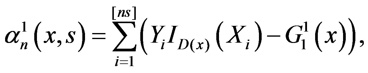
Proof of Corollary 3: Assume the alternative Hypothesis (2). Then,
where, for s < θ,
and for ,
,
with
and
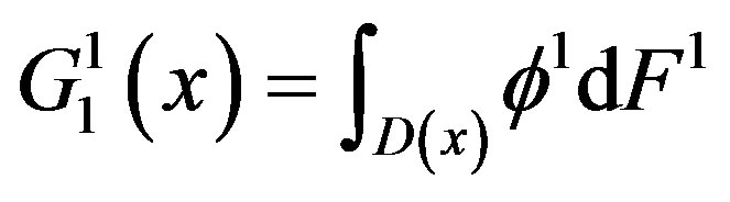 .
.
If Condition (A3) holds for the functions ϕ1 and F1, then under the alternative Hypothesis (2),
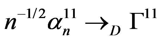 in the space
  with the uniform metric, where Г11 is a zero-mean Gaussian process. Strong consistency of the statistics nKS, nKC, nMC follows. (See the proof of Theorem 4.1 in [5]).
Proof of Theorem 4: Let
 .
.
By the multivariate CLT, along almost all sequences,
 ,
,
is a sum of iid random variables with mean zero and a resulting covariance matrix having entries of the form
which converge, uniformly in (x1, s1) and (x2, s2),
 .
.
Similarly, the corresponding conditional covariance of
converges uniformly to
 and the corresponding conditional covariance of
  converges uniformly to that of Г.
By the multiplier inequalities ([12], Lemma 3.6.7),

where  is uniformly distributed on the set of all permutations of
  and is independent of
 . In our case,
  is the collection of functions
 .
.
also,
denotes (uniform) measurable covers with respect to all variables jointly. Using Theorem 1, as in the proof of Theorem 3.6.13 in [12], x n(x, 1) is Donsker. It follows that ([12], Theorem 2.12.2) xn(x, s) is Donsker, and Theorem 4 for b(j) follows.
Proof of Theorem 5: The proof is similar to that of Theorem 4 but where the limiting covariance of is that of G11 instead of Г.
6. Concluding Remarks
In this paper, we have constructed test statistics using
 the lower orthants. It is clear (see [12]) that other Donsker classes of functions can be used. Examples are: the collection of the closed balls, or the collection of half-spaces. The method of proof in [5,6,15] could not handle such classes. One can also obtained weak convergence of the weighted version of the process where the weight functions satisfy the Chibisov-O’Reilly conditions (see [5,6], or [16], p. 462).
The simulations show that our tests have good power considering the omnibus nature of the procedure. By avoiding curve estimation (e.g. using kernel methods to estimate f), we are able to provide practical tests for moderate sample sizes.
REFERENCES
- C. Lee,M. Csörgő and L. Horváth, “Limit Theorems in Change-Point Analysis,” Wiley, Chichester, 1997.
- M. Csörgő, L. Horváth and B. Szyszkowicz, “Integral Tests for Suprema of Kiefer Processes with Application,” Statist, Decisions, Vol. 15, No. 4, 1997, pp. 365-377.
- M. Csörgő and B. Szyszkowicz, “Weighted Multivariate Empirical Processes and Contiguous Change-Point Analysis,” Change-Point Problems, IMS Lecture Notes Monograph Series, Vol. 23, 1994, pp. 93-98. doi:10.1214/lnms/1215463116
- M. Csörgő and B. Szyszkowicz, “Applications of MultiTime Parameter Processes to Change-Point Analysis, In: M. Fisz, Ed., Probability Theory and Mathematical Statistics, John Wiley & Sons, Inc., New York, 1994, pp. 159-222.
- M. D. Burke, “Limit Theorems for Change-Point Detection in Nonparametric Regression Models,” Acta Mathematica (Szeged), Vol. 73, No. 3-4, 2007, pp. 865-882.
- M. D. Burke, “Approximations for a Multivariate Hybrid Process with Applications to Change-Point Detection,” Mathematical Methods of Statistics, Vol. 19, No. 2, 2010, pp. 121-135. doi:10.3103/S106653071002002X
- M. D. Burke, “A Gaussian Bootstrap Approach to Estimation and Tests,” In: B. Szyszkowicz, Ed., Asymptotic Methods in Probability and Statistics, Elsevier, Amsterdam, 1998, pp. 697-706. doi:10.1016/B978-044450083-0/50045-9
- M. D. Burke, “Multivariate Tests-of-Fit and Uniform Confidence Bands Using a Weighted Bootstrap,” Statistics and Probability Letters, Vol. 46, No. 1, 2000, pp. 13-20. doi:10.1016/S0167-7152(99)00082-6
- D. Pollard, “A Central Limit Theorem for Empirical Processes,” Journal of the Australian Mathematical Society A , Vol. 33, No. 2, 1982, pp. 235-248. doi:10.1017/S1446788700018371
- E. Giné and J. Zinn, “Bootsrapping General Empirical Measures,” Annals of Probability, Vol. 18, No. 2, 1984, pp. 851-869. doi:10.1214/aop/1176990862
- E. Giné and J. Zinn, “Lectures on the Central Limit Theorem for Empirical Processes,” Lecture Notes in Mathematics, Vol. 1221, 1986, pp. 50-113. doi:10.1007/BFb0099111
- A. W. Van der Vaart and J. A. Wellner, “Weak Convergence and Empirical Processes: With Applications to Statistics,” Springer, New York, 1996. doi:10.1007/978-1-4757-2545-2
- B. G. Ivanoff, “Stopping Times and Tightness for Multiparameter martingales,” Statistics & Probability Letters, Vol. 28, No. 2, 1996, pp. 111-114. doi:10.1016/0167-7152(95)00103-4
- M. D. Burke, “Testing Regression Models: A Strong Martingale Approach,” Fields Institute Communications. 2004.
- L. Horváth, “Approximations for hybrids of empirical and partial sums processes,” Journal of Statistical Planning and Inference, Vol. 88, No. 1, 2000, pp. 1-18. doi:10.1016/S0378-3758(99)00207-4
- G. R. Shorack and J. A. Wellner, “Empirical Processes with Applications to Statistics,” Wiley, New York, 1986.
NOTES
*Corresponding author.