Open Journal of Statistics
Vol.3 No.3(2013), Article ID:33242,13 pages DOI:10.4236/ojs.2013.33023
Sampling Error Estimation in Stratified Surveys
Department of Mathematics, Campus de Elviña, University of A Coruña, A Coruña, Spain
Email: juan.vilar@udc.es
Copyright © 2013 Ricardo Cao et al. This is an open access article distributed under the Creative Commons Attribution License, which permits unrestricted use, distribution, and reproduction in any medium, provided the original work is properly cited.
Received March 7, 2013; revised April 8, 2013; accepted April 15, 2013
Keywords: Variance Estimation; Jackknife; Bootstrap; Stratified Sampling
ABSTRACT
Many operations carried out by official statistical institutes use large-scale surveys obtained by stratified random sampling without replacement. Variables commonly examined in this type of surveys are binary, categorical and continuous, and hence, the estimates of interest involve estimates of proportions, totals and means. The problem of approximating the sampling relative error of this kind of estimates is studied in this paper. Some new jackknife methods are proposed and compared with plug-in and bootstrap methods. An extensive simulation study is carried out to compare the behavior of all the methods considered in this paper.
1. Introduction
Many of the operations carried out by official statistics institutions are based on surveys performed on a finite population using stratified random sampling without replacement. These surveys provide information on three types of variables: binary, categorical with more than two modalities, and continuous quantitative variables. Usually, most of the variables are binary, i.e. they yield two possible responses commonly coded with 1 and 0, and the aim is to estimate . A typical example is the variable indicating the presence or absence of a particular characteristic of interest in the study population, e.g. if a person is employed or unemployed, a household has Internet access or not, etc. In the case of categorical variables with more than two possible responses, say
 , the aim is to estimate the proportion of each of the answers,
 . For continuous quantitative variables,
  , the objective is to estimate the mean of the variable,
 .
.
Stratified sampling is an appropriate method when several homogeneous and mutually exclusive strata or subpopulations are identified in the population. Stratification can contribute to improve the representativeness of the sample by reducing sampling error. The bigger the differences between the strata, the greater the gain in accuracy. Moreover, some strata can be occasionally small in size but big in importance in the study. In these cases, an exhaustive sampling is recommended, i.e. all the individuals of these strata will be part of the sample. These strata are called self-represented.
Once that a population quantity , such as a mean or a proportion, has been estimated, it is important to obtain an accurate estimate of the sampling error to assess the reliability of our estimator
 . The sampling error of
  can be presented in absolute terms, using the standard deviation of
 , namely
or in relative terms, using the variation coefficient of the estimator given by
This work addresses the problem of estimating sampling errors in surveys carried out by stratified sampling from finite populations. Some new proposals to obtain sampling relative error estimates are introduced and various methods based on plug-in, jackknife and bootstrap techniques are compared. This research originated from the collaboration with the Galician Official Statistical Institute (IGE), the agency in charge of the official statistics in the Autonomous Community of Galicia, a region in the Northwest of Spain. Specifically, IGE was interested in assessing different criteria to approximate the sampling relative error for a variety of statistics produced by the Annual Company Survey (ACS), which is conducted by IGE in Galicia.
About 200 variables are recorded in the Galician ACS, a survey including nearly 4000 companies in a total population of 65,000. The sample is obtained by stratified random sampling, with strata having different weights and some of them being self-represented. The strata are constructed by regarding the combination of three variables: the level of research performed in the company, the size of the company, measured in terms of the number of paid employees, and the main activity of the company.
The rest of this work is divided into the following sections. Notation used some basic concepts are introduced in Section 2. Section 3 describes the different jackknife procedures used to estimate the relative error of the estimators. The bootstrap methods of the error estimation are described in Section 4. Some results from a broad simulation study carried out to compare the behaviour of all the methods studied are presented in Section 5. Finally, the main conclusions of the work are established in Section 6.
2. Notation and Basic Concepts
From now on,  and
and  will denote the population size, the number of strata and the population size of the i-th stratum,
  , respectively. Given a variable of interest,
  ,
,  is the j-th element of the i-th population stratum, with
 . When the variable in study is quantitative (continuous or discrete), it will make sense to speak about the population mean,
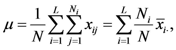 (2.1)
(2.1)
and the population total,
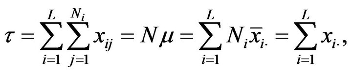 (2.2)
(2.2)
being  and
and .
.
Let  be a stratified random sample without replacement of
 , of size
 ,
,  being the sample size within the
  -th stratum. Denoting by
  the elevation factors of each stratum, the unbiased estimators of the mean
  and the total
 ![]() are obtained as follows.
are obtained as follows.
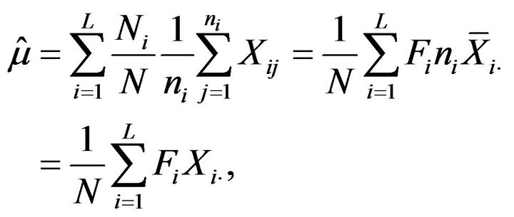 (2.3)
(2.3)
and
 (2.4)
(2.4)
where 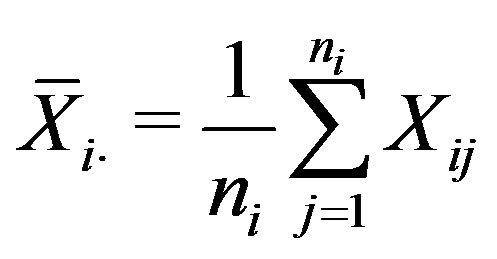 and
and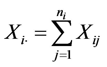 .
.
Note that, by definition,  for the strata selfrepresented in the sample, and hence the elevation factor of these strata is
 .
.
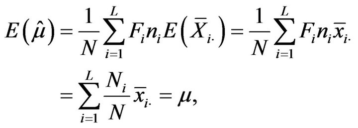
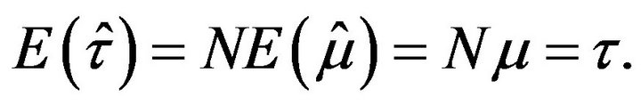
The unbiasedness property of  and
and  as estimators of
  and
and![]() , respectively, follows from its construction as convex linear combinations of sample means (see (2.3) and (2.4)). So, from (2.1) and (2.2) follows
, respectively, follows from its construction as convex linear combinations of sample means (see (2.3) and (2.4)). So, from (2.1) and (2.2) follows
and
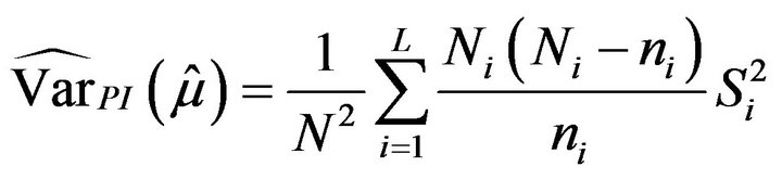
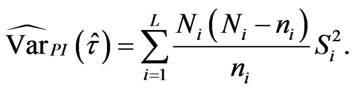
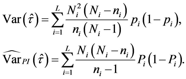
Some simple calculations, although long (see, for example, [1]), yield the variance of these estimators. Specifically,
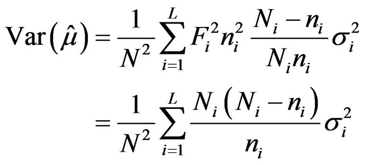 (2.5)
(2.5)
and
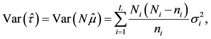 (2.6)
(2.6)
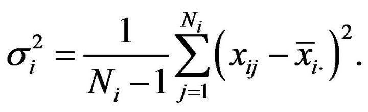
 being the variance of the finite population in the i-th stratum, given as
Replacing the population variances , in (2.5) and (2.6) by the corresponding sample variances corrected by their degrees of freedom,
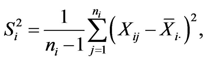
we obtain plug-in estimators for the variance of  and
and . Specifically,
 (2.7)
(2.7)
In the particular case of a binary variable we have
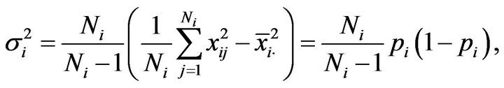
that is estimated using
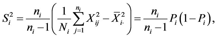
where  denotes the true proportion of ones in the
  -th stratum and
  the corresponding sampling proportion. Using the new expressions for
  and
and  in (2.6) and (2.7), respectively, we obtain the variance of
  and its plug-in estimator for binary variables, which are reduced to
Going back to the general case in (2.5), it is deduced that the absolute and relative sampling errors of estimator  take the form
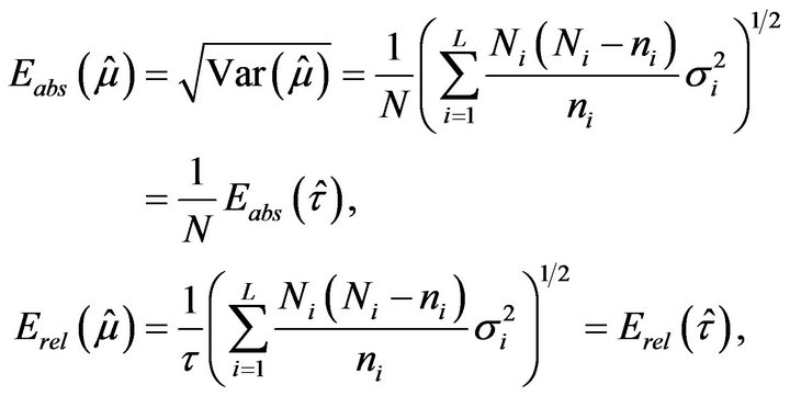
Hence, the plug-in estimators of these errors are
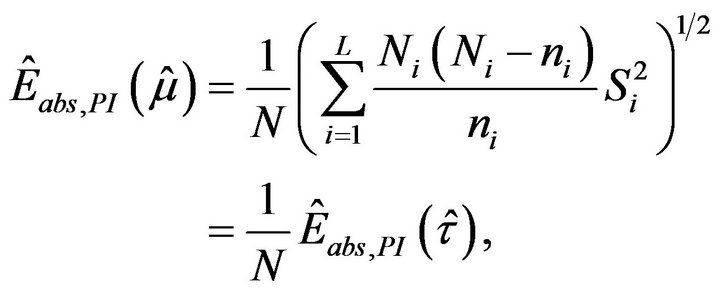 (2.8)
(2.8)
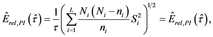 (2.9)
(2.9)
As  and
and , the relative errors of
  and
and  as well as of their estimations are the same. Hence, the rest of the study will focus on the estimation of the relative error of parameter
![]() , the population total.
, the population total.
3. Jackknife Estimation
The jackknife method is a general estimation procedure introduced by [2] that has been widely used to estimate the bias and the standard error of a statistic. It is well known that the jackknife technique leads to a reduction in the bias. Furthermore, the jackknife method is basically a resampling procedure, and hence one can estimate the accuracy of an estimator without assuming previous hypotheses on the distribution of the population.
Let  be an estimator of a parameter
  based on the sample
 , then the jackknife estimator of the variance of
  is defined as
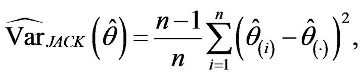
where ![]() is the jackknife pseudovalue, that is the estimator calculated using the whole sample except for the i-th observation,
is the jackknife pseudovalue, that is the estimator calculated using the whole sample except for the i-th observation,  , and
, and ![]() is the mean of the jackknife pseudovalues,
is the mean of the jackknife pseudovalues,
 .
.
In a stratified sampling, the jackknife pseudovalues can be constructed following one of the two possible criteria: either removing a sample value at each iteration or removing a stratum at each iteration. Application of these criteria leads to two different jackknife estimators for the variance of  and
and . Moreover, according to (2.4),
  can be expressed as a linear combination of independent statistics
 , each one being separately constructed from the subsample of each stratum. Consequently, the variance of
  can be calculated as a linear combination of variances of statistics constructed at stratum level. If these variances are previously estimated by jackknife in each stratum, then there will be a third way of using the jackknife to approximate the variance of
 . Each of the three jackknife proposals are described more in detail below.
3.1. Jackknife Leaving One Sample Value out
Each jackknife pseudovalue is constructed by removing a single data value from the overall sample
 . Thus, the pseudovalue obtained when eliminating the s-th observation of the r-th stratum,
  , takes the form
where 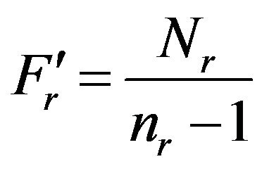 and
and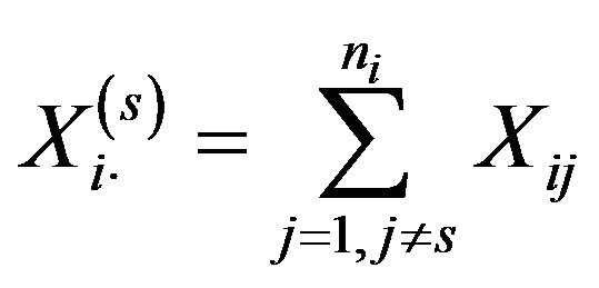 .
.
On the other hand we have that
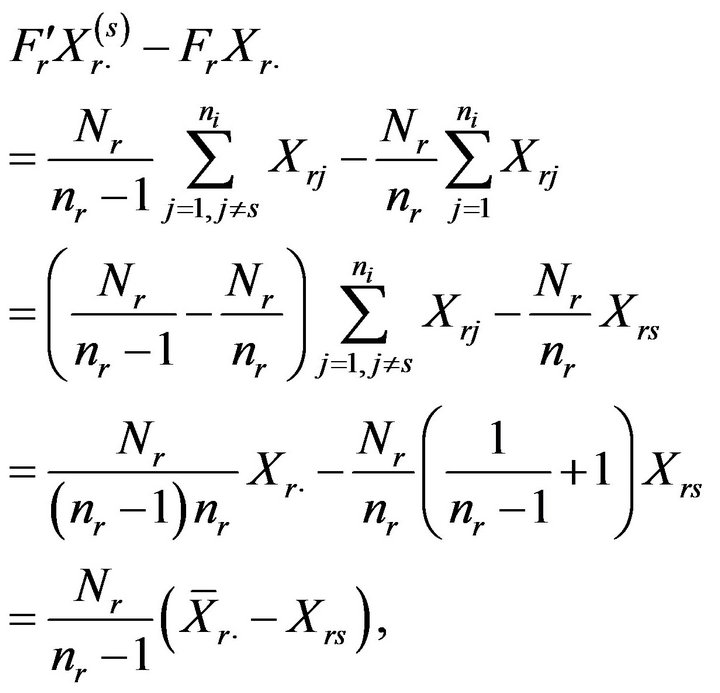
and hence

By averaging all the pseudovalues, we obtain
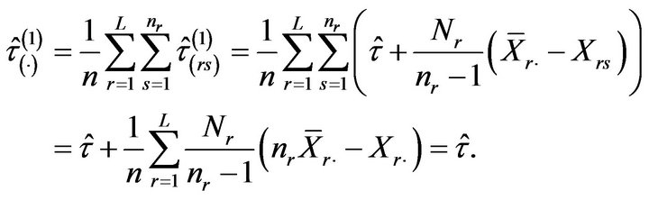
Hence, the jackknife estimator of  is given by
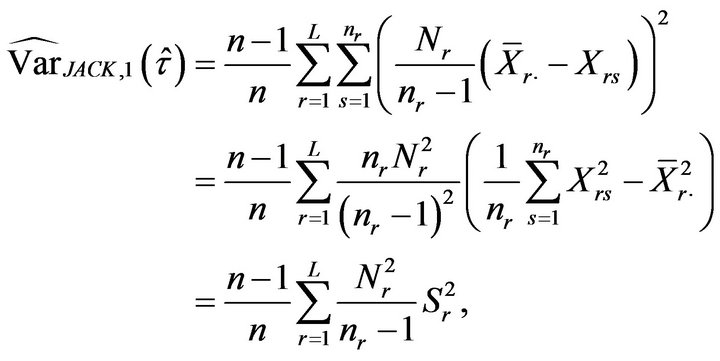
and the first variant of the jackknife estimator for the relative error is
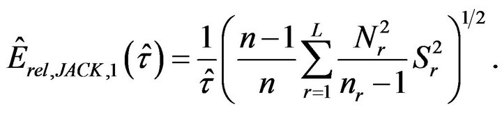 (3.1)
(3.1)
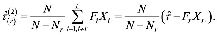
3.2. Jackknife Leaving One Stratum out
Here we propose to calculate each pseudovalue removing all the observations of one stratum. Thus, the  -th jackknife pseudovalue is based on the original sample without the observations of stratum
 , i.e.
Now, two variants of the jackknife estimator are introduced by considering different ways of averaging the pseudovalues . First, we use a weighted mean, where each pseudovalue is weighted by the population size of the stratum removed in the calculation. Thus, we have
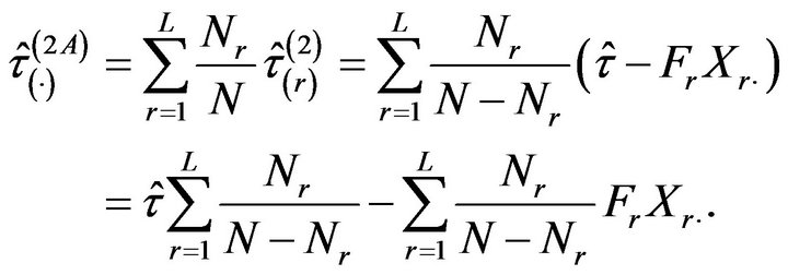
Then, the jackknife estimator of  takes the form

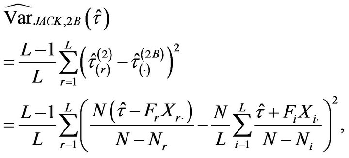
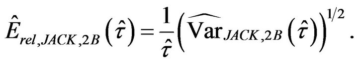
Note that, in this case, it seems that a more simplified expression cannot be achieved. The jackknife estimator of the relative error is then calculated as
 (3.2)
(3.2)
An alternative variant of the jackknife leaving a stratum out is obtained if all the strata contribute with the same weight in the estimation, i.e. the pseudovalues are directly averaged as follows
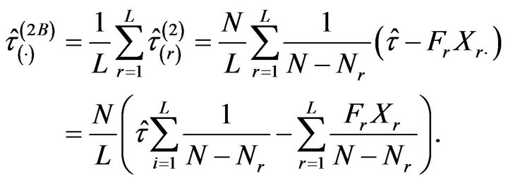
Using , the jackknife estimator of
  becomes
not admitting a simpler explicit expression either.
The jackknife estimator of the relative error with this criterion is
 (3.3)
(3.3)
3.3. Jackknife within Each Stratum
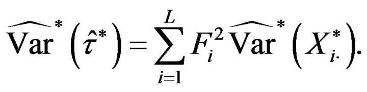
According to (2.4), the variance of  can be expressed as a linear combination of the variances of the sample means within each stratum
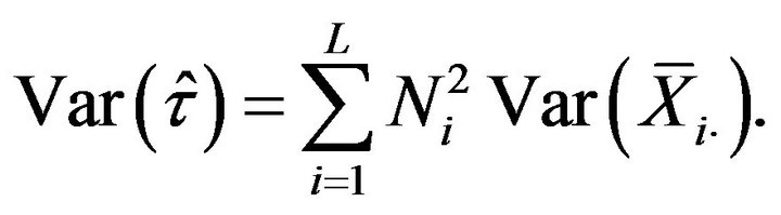 (3.4)
(3.4)
Hence, a new jackknife approximation to the variance of  can be obtained by estimating each
  with the jackknife method and replacing these estimators in (3.4). For the jackknife estimator of
 , the pseudovalues are defined as

for , and their mean is given by
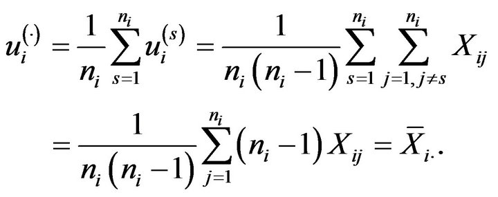
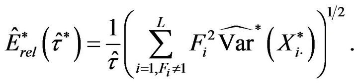
Then, the jackknife estimator of the variance of the sample mean of the i-th stratum is
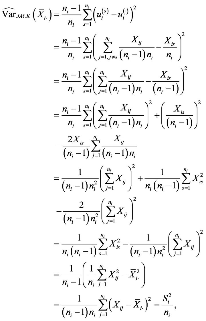
and using these previous jackknife estimations we obtain
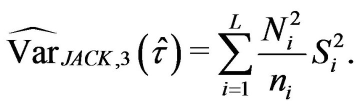
The corresponding jackknife estimation of the relative error is given by
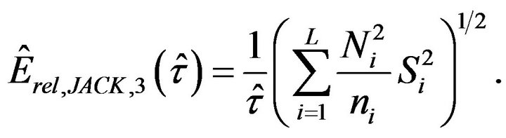 (3.5)
(3.5)
4. Bootstrap Estimation
An alternative resampling method often used to estimate the variance and the relative sampling error of the estimators is the bootstrap or self-sufficient estimation method. As any resampling procedure, including jackknife, the bootstrap takes advantage of not requiring hypotheses on the underlying distribution. The bootstrap method was introduced by Efron (see [3-5]) and has been widely treated in the literature. The basic idea of bootstrap consists in estimating the underlying population and then drawing out a number of resamples from the estimated population. By extracting a large number  of these resamples (in the order of one or several thousand),
  bootstrap replications of a particular estimator
  can be obtained and used to approximate the estimator variance and relative error.
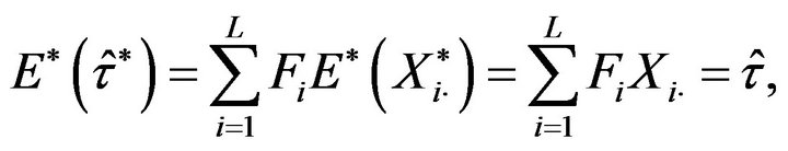
According to (2.4), the estimator  can be written as the sum of the independent random variables
 . Hence, the bootstrap can be either applied to the global population, in order to directly estimate the variance of
 , or to each of the strata, in order to estimate the variance of each statistic
  and then approximate the variance of
  as the sum of the variances of
 . In particular, any bootstrap resampling plan ensuring the independence among different strata is valid to be used on the whole sample or stratum by stratum, although the latter is indeed more efficient computationally. Note also that the statistic
  will have zero variance in self-represented strata, where the sampling is exhaustive
 , and therefore it is not necessary to draw out bootstrap resamples in these strata.
A detailed description of two bootstrap resampling procedures to approximate the population total in a fixed stratum , with
 , is provided below.
4.1. Bickel and Freedman Bootstrap Method
The proposal by Bickel and Freedman (see [6]) consists in estimating the underlying population from a mixture of two distinct and equal-sized finite populations.
If  is an integer number, then the bootstrap algorithm proceeds as follows.
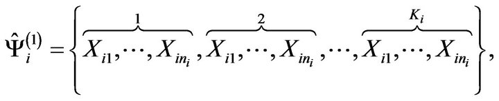
BF.1 The estimated subpopulation for the i-th stratum is constructed by grouping  identical copies of the sample of the stratum, that is the empirical population is given by
BF.2 A bootstrap resample of size ,
,  is selected at random and without replacement from
 .
.
BF.3 A bootstrap estimate for the population total in the i-th stratum,  , is calculated from the bootstrap resample derived in the previous step.
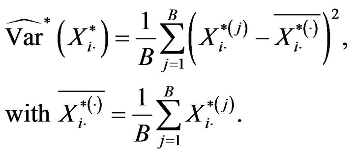
BF.4 Steps BF.2 and BF.3 are repeated a large number,  , of times (
 or 5000, for example), thereby obtaining a set of
  bootstrap replicates of the total estimator,
 . Then, the bootstrap variance of the total,
  , is approximated by means of
 (4.1)
(4.1)
When the elevation factor  is not integer, Steps BF.1 and BF.2 are modified as follows.
BF.1’ Consider , being
 , where
  denotes the integer part function. Thus,
  , with
  and
and .
.
Two empirical finite subpopulations  and
and ![]() are now considered for the i-th stratum, which are formed, respectively, by
are now considered for the i-th stratum, which are formed, respectively, by  and
and  identical copies of the observed sample, that is
BF.2’ Define . A bootstrap resample of size
 , is selected randomly and without replacement from
  with probability
 , and from
 ![]() with probability
with probability .
.
The specific selection of  ensures that the mean and the variance in the resampling of a bootstrap observation
  are equal to the expected quantities when the size of the bootstrap population is
 . Notice that the first resampling algorithm is a particular case of the previous one. In fact, if
  is an integer, i.e. Ri = 0, then
  and both algorithms become identical.
4.2. Booth, Butler and Hall Bootstrap Method
The bootstrap procedure proposed by Booth, Butler and Hall (see [7]) is based on completing the population  estimated in Step BF.1’ by adding a random subsample of the observed sample. In this way, one avoids using the two finite bootstrap populations
  and
and![]() . More precisely, Steps BF.1’ and BF.2’ of the Bickel and Freedman algorithm are modified as follows.
. More precisely, Steps BF.1’ and BF.2’ of the Bickel and Freedman algorithm are modified as follows.
BBH.1 As in Step BF.1’, consider , where
  and
and , with
 .
.
The finite subpopulation estimated for the i-th stratum is given by , where
  is constructed as in Step BF.1’, i.e.
and ![]() is formed by a random subsample of size
is formed by a random subsample of size  generated without replacement from
 .
.
BBH.2 A bootstrap resample of size is selected at random and without replacement from
![]() .
.
The bootstrap estimation of the variance of the statistic  is now obtained using (2.4) and the bootstrap approximations
  calculated with one of the algorithms previously described. Specifically,
Considering that
the bootstrap relative error is given by
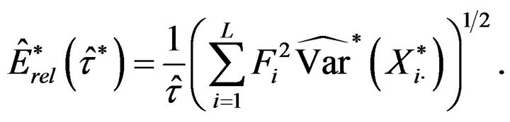 (4.2)
(4.2)
Note that the bootstrap variance for an exhaustive stratum is equal to zero, and hence the sum in (4.2) can be restricted to the non-exhaustive strata. Thus, we can write
This clearly reduces the computational effort because no bootstrap resamples are generated from self-represented strata.
5. Simulation Study
An extensive simulation study was performed to compare the estimators of the relative error of the population mean,  , described in the previous sections. Specifically, the following estimators
 ![]() were computed: the plug-in estimator
were computed: the plug-in estimator  given in (2.9); the jackknife estimators
  (leaving out one value),
  and
and  (both leaving out one stratum), and
  (jackknife in each stratum) given in (3.1), (3.2), (3.3) and (3.5), respectively; and the bootstrap estimators derived from (4.1) using the resampling algorithms by Bickel and Freedman (BF estimator) and by Booth, Butler and Hall (BBH estimator).
As the self-represented strata do not affect to the sampling error, corrected versions of the jackknife estimators were also constructed by omitting the pseudovalues associated with these strata. These corrected versions are referred as the original ones but adding the letter “C”. Note that this correction is implicit by construction in the case of the plug-in and bootstrap estimators.
Three different types of response variables were simulated in our experiments:
Binary variables. The response is “1” or “0” and the parameter of interest is , which was chosen to take values close to 0.50, 0.30, 0.15 and 0.05.
Multinomial variables. Variables taking four possible results denoted by  and
and  were considered. Here, the parameter of interest is the vector
 , with
 , for
, for . Specifically,
 ![]() was selected to take the value
was selected to take the value .
.
Continuous variables. Response variables generated from three possible absolutely continuous distributions: uniform, normal and exponential.
Different scenarios of high and low variability between the mean responses of the population strata were simulated. In all our experiments, the population size was  data values, classified in
  strata so that two of these strata were self-represented in the sampling. The first experiments were carried out with a sample size
 . Thus, the ratio between the sample and population sizes mimics the one in the Galician ACS conducted by IGE and that initially motivated the present work.
Our first results come from an experiment with binary response. The specific parameter values used to generate the population and the sample are shown in Table 1.
Table 1 summarizes the main features of the experiment. Thus, for instance, stratum L1 is formed by 1200 observations taking two possible values, “0” and “1”, that have been randomly generated from Bernoulli trials with . Note that all the values
  are around 0.5, but there is a high variability between them. The overall population consists of 5000 observations and satisfies that
  and
and .
.
Under this population design,  samples of size
  were generated, and hence 1000 estimates
 ![]() were obtained with each studied method. In the case of the bootstrap procedures, a set of
were obtained with each studied method. In the case of the bootstrap procedures, a set of  bootstrap
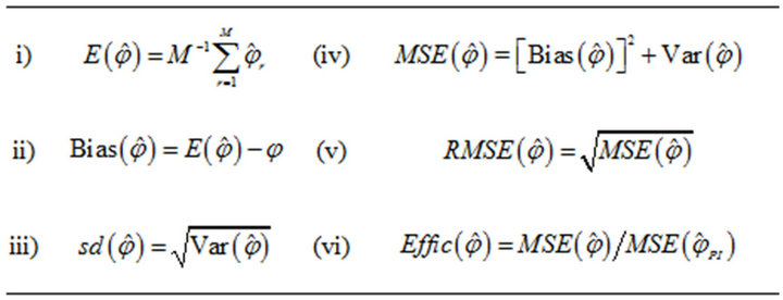
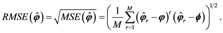
replicates was considered to compute each estimator. The behaviour of each estimation procedure was examined by using the following values:
The quantity  measures the efficiency of each estimator
 ![]() with respect to the plug-in estimator,
with respect to the plug-in estimator, . Thus,
  means that the considered estimator
 ![]() presents better behavior than the plug-in estimator in terms of mean squared error. Results from our first experiment are shown in Table 2, where different scales have been used to obtain a more intuitive comparison.
presents better behavior than the plug-in estimator in terms of mean squared error. Results from our first experiment are shown in Table 2, where different scales have been used to obtain a more intuitive comparison.
Similar experiments were carried out using different sample sizes , where the new sample size in the i-th stratum,
  , was determined by
 , with
  being the sample size of the first experiment (see Table 1) and k = 0.25, 0.30, 2, 3 and 4. Excluded from this rule are the two self-represented strata for which obviously
  in all cases. The values of
  and
and  obtained with these new sample sizes are presented in Tables 3 and 4, respectively.
New trials of our first experiment were run with different values of parameter . Table 5 presents results of
  obtained for different values of
![]() .
.
Tables 2-5 provide a sample of the results obtained in our extensive numerical study with binary response. Some interesting conclusions derived from this study are stated below.
• The plug-in method gave good results and was often the most efficient procedure. Moreover, it has the advantage of being computationally fast. It is also observed that its efficiency improves with increasing sample size.
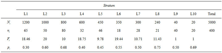
Table 1. Parameters in the first experiment with binary response: population size , sample size
 , elevation factor
  and
and  for the i-th stratum
 .
.
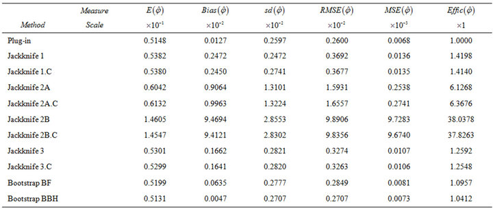
Table 2. Results for the experiment with binary response conducted under parameters in Table 1. Total population parameters:  and
and . Results based on
  trials with sample size
 .
.
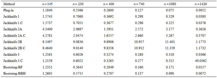
Table 3. Values of  for different sample sizes.
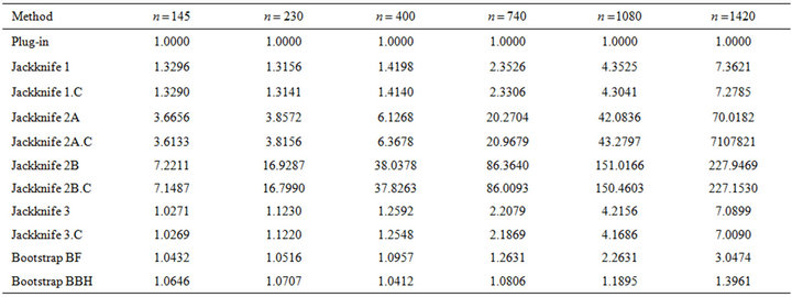
Table 4. Results of  for different sample sizes.
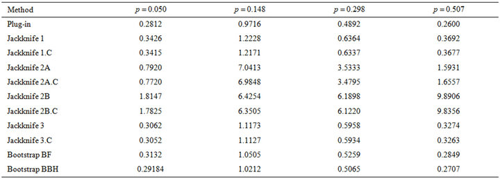
Table 5. Results of  for different values of
 .
.
• Both bootstrap methods (BF and BBH) yield competitive results. The BBH bootstrap presents better behaviour than the BF bootstrap, especially for large sample sizes. For moderate or small sample sizes (less than 10% of the population size), the bootstrap methods behave similarly to the plug-in method in terms of efficiency, although with a higher computational cost (that, in any case, results to be acceptable).
• The jackknife 3 estimator (based on applying jackknife to each stratum) behaved similarly to the bootstrap estimators for small sample sizes  and worsened with increasing
![]() . Jackknife 1 estimator (based on leaving out one sample datum) was competitive although yielded worse results than the jackknife 3 with small sample sizes. Both variants of the jackknife 2 estimator (based on leaving out one stratum) yielded much worse results for all the considered sample sizes. Therefore, it is not advisable to use the jackknife 2 estimators. In general, the worse behaviour of the jackknife-based estimators seems to be mainly due to the bias of the estimation, although for the jackknife 2 estimators poor results are also observed in terms of standard deviation.
. Jackknife 1 estimator (based on leaving out one sample datum) was competitive although yielded worse results than the jackknife 3 with small sample sizes. Both variants of the jackknife 2 estimator (based on leaving out one stratum) yielded much worse results for all the considered sample sizes. Therefore, it is not advisable to use the jackknife 2 estimators. In general, the worse behaviour of the jackknife-based estimators seems to be mainly due to the bias of the estimation, although for the jackknife 2 estimators poor results are also observed in terms of standard deviation.
• No substantial differences were observed between using the jackknife procedures and their corrected versions (.C), based on cancelling the exhaustive strata. Just a slight advantage for the corrected versions is observed.
• Similar conclusions are valid for the two scenarios of high and low variability of the response between different strata. In general, the plug-in estimator is the most efficient in both situations, although the differences between the plug-in and the other methods are smaller in the case of low variability.
• For small sample sizes , both two bootstrap methods and jackknife 3 led to a greater efficiency than the plug-in method.
• Results in Table 5 allows us to conclude that prior comments are valid for binary variables regardless of the specific value taken by . In particular, it is observed that
  takes the smallest values when
 ![]() is close to 0 or 0.5.
is close to 0 or 0.5.
Next step in our simulation study is addressed to analyze the case of multiple response. Specifically, it is assumed that there are four mutually exclusive and exhaustive results for the response variable, let us say  and
and . As in the case of binary response, a population of
  observations divided in L = 10 strata was simulated. Data forming the
  -th stratum were randomly generated from a multinomial distribution with parameter
 , where
  denotes the probability of event
  in the
  -th stratum,
 . Different values of
  were selected to set up scenarios with high and low variability of the responses between strata. In all cases, the overall population, which is formed by bringing together all strata, presents the theoretical parameter vector
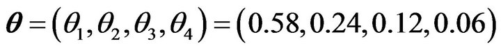 , where
 .
.
A total of  samples of size
  were randomly selected and each of them was used to construct an estimator
 ![]() of the relative error in the sampling of
of the relative error in the sampling of . Again, two strata were considered to be exhaustive in the sampling. The theoretical error for the simulated population is
 . The set of estimates obtained with each of the studied methods
  is then used to calculate the mean squared error and the efficiency of each procedure with respect to the plug-in method. Both quantities were simultaneously obtained for each estimated marginal component
  and jointly for the estimated vector
 . In particular, the global
  is given by
Results from this new simulation are shown in Tables 6 and 7.
Results from Tables 6 and 7 show that the conclusions derived from simulations with binary response are equally valid for the case of multiple response.
Finally, we focus on the case of continuous response variables. Thus, new experiments were carried out to examine the performance of the different estimation procedures with responses generated from uniform, normal and exponential distributions. The simulation plan was designed by following the same outline as in previous experiments.
For instance, some experiments with normal and exponential responses were carried out considering the features summarized in Table 8. Note that these parameters lead to a situation of high variability between data from different strata. Some outcomes derived from these experiments are presented in Tables 9 and 10, for the Gaussian case, and in Tables 11 and 12, for the exponential case. Here, the target parameter in the overall population,  , took the value
  for the Gaussian response, and
 , for the exponential response.
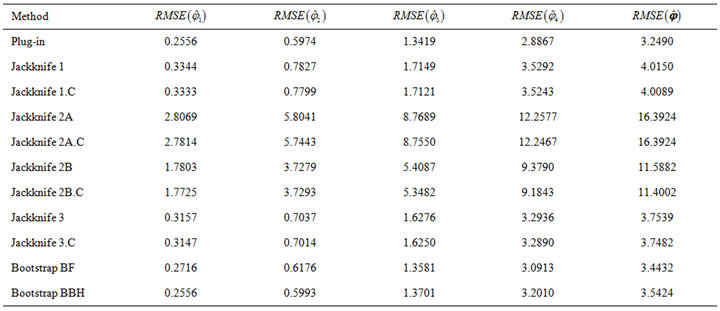
Table 6. Results of  for the experiment with multiple response and high response variability between strata. Results based on
  trials with sample size
 .
.
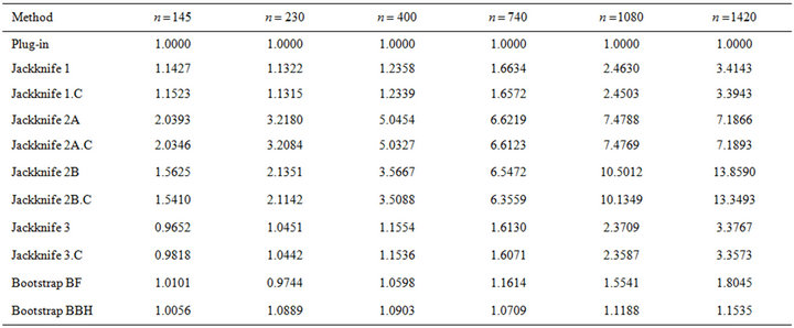
Table 7. Results of  for the experiment with multiple response and high response variability between strata. Results based on
  trials with sample size
 .
.
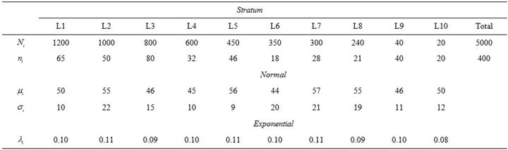
Table 8. Main features for experiments with normal and exponential responses: population size , sample size
  and distribution parameters for the
  -th stratum
![]() .
.
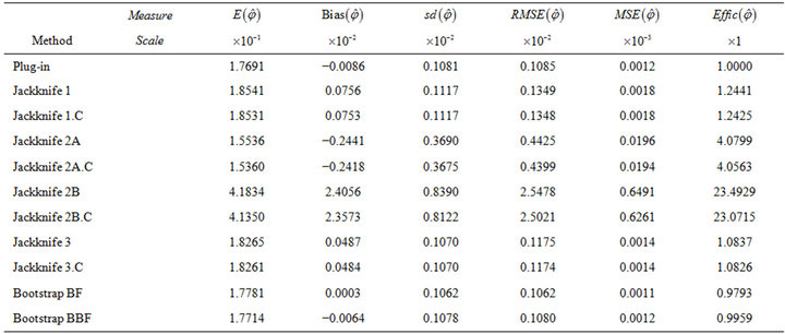
Table 9. Results from the experiment with Gaussian response conducted according to parameters in Table 8 and based on  trials with sample size
 .
.

Table 10. Results of  for Gaussian response and different sample sizes.
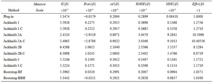
Table 11. Results from the experiment with Exponential response conducted according to parameters in Table 8 and based on M = 1000 trials with sample size n = 400.

Table 12. Results of  for exponential response and different sample sizes.
Results in Tables 9-12 allow us to confirm that the different analyzed estimation procedures behaved as in the previous experiments. Moreover, an analogous behaviour was also observed with uniform response and with scenarios of low variability between strata. In short, the conclusions derived from our numerical study with binary or multinomial response can be extended to the case of continuous response variables, regardless of the generating probability distribution.
6. Final Conclusion
The present work deals with the problem of estimating the sampling relative error of point estimates derived from large sample surveys. It is specifically assumed that the survey’s sampling design is the stratified random sampling without replacement, because this design is often considered in many surveys conducted by different official statistics institutions. Variables commonly examined in this type of surveys are binary, categorical and continuous, and hence, the estimates of interest involve estimates of proportions, totals and means. In this setting, several procedures to approximate the sampling relative error of this kind of estimates are proposed. Different estimation techniques are considered, including the natural estimation of plug-in type and more sophisticated methods based on jackknife and bootstrap methodologies. The behaviour of the different procedures proposed is examined and compared by means of an extensive simulation study. In general, the plug-in method presents good behaviour in all the analyzed situations, with the additional advantage of having a low computational cost. For small sample sizes, the jackknife estimator denoted by “jackknife 3”, which is based on the prior application of the jackknife technique to each stratum, and the two bootstrap methods considered (particularly the bootstrap proposed by Booth, Butler and Hall) yield results similar as those obtained with the plug-in estimator, and in some cases, even better. However, the estimators obtained with these methods have a higher (although acceptable) computational cost.
7. Acknowledgements
This research was supported by the Galician Official Statistical Institute (IGE) and by Grants 10DPI105003PR and CN2012/130 from Xunta de Galicia (Spain), and by Grant number MTM2011-22392 from Ministerio de Ciencia e Innovación (Spain).
REFERENCES
- S. K. Thompson, “Sampling,” Wiley, New York, 1992.
- M. Quenouille, “Approximate Tests of Correlation in Time Series,” Journal of the Royal Statistical Society: Series B (Statistical Methodology), Vol. 11, No. 1, 1949, pp. 18-84.
- B. Efron, “Bootstrap Methods: Another Look at the Jackknife,” The Annals of Statistics, Vol. 7, No. 1, 1979, pp. 1-26. doi:10.1214/aos/1176344552
- B. Efron, “The Jackknife, the Bootstrap, and Other Resampling Plans, Siam Monograph 38,” Society of Industrial and Applied Mathematics CBMS-NSF Monographs, 1982.
- B. Efron and R. Tibshirani, “An Introduction to the Bootstrap,” Chapman & Hall, New York, 1993.
- P. J. Bickel and D. A. Freedman, “Asymptotic Normality and the Bootstrap in Stratified Sampling,” The Annals of Statistics, Vol. 12, No. 2, 1984, pp. 470-482. doi:10.1214/aos/1176346500
- J. G. Booth, R. W. Butler and P. Hall, “Bootstrap Methods for Finite Populations,” Journal of the American Statistical Association, Vol. 89, No. 248, 1994, pp. 1282- 1289. doi:10.1080/01621459.1994.10476868