Open Journal of Statistics
Vol.1 No.3(2011), Article ID:8070,13 pages DOI:10.4236/ojs.2011.13021
A Kullback-Leibler Divergence for Bayesian Model Diagnostics
1Department of Epidemiology and Biostatistics, University of Texas Health Science Center, San Antonio, USA
2Department of Statistics, University of Florida, Gainesville, USA
E-mail: wangc3@uthscsa.edu, ghoshm@stat.ufl.edu
Received August 18, 2011; revised September 19, 2011; accepted September 29, 2011
Keywords: Kullback-Leibler Distance, Model Diagnostic, Weighted Posterior Predictive p-Value
Abstract
This paper considers a Kullback-Leibler distance (KLD) which is asymptotically equivalent to the KLD by Goutis and Robert [1] when the reference model (in comparison to a competing fitted model) is correctly specified and that certain regularity conditions hold true (ref. Akaike [2]). We derive the asymptotic property of this Goutis-Robert-Akaike KLD under certain regularity conditions. We also examine the impact of this asymptotic property when the regularity conditions are partially satisfied. Furthermore, the connection between the Goutis-Robert-Akaike KLD and a weighted posterior predictive p-value (WPPP) is established. Finally, both the Goutis-Robert-Akaike KLD and WPPP are applied to compare models using various simulated examples as well as two cohort studies of diabetes.
1. Introduction
Information theory provides a general framework of developing statistical techniques for model comparison (Akaike [2]; Shannon [3]; Kullback and Leibler [4]; Lindley [5]; Bernardo [6]; Schwarz [7]). The KullbackLeibler distance (KLD) is perhaps the most commonly used information criterion for assessing model discrepancy (Akaike [2]; Kullback and Leibler [4]; Lindley [5]; Schwarz [7]). In essence, a KLD is the expected logarithm of the ratio of the probability density functions (p.d.f.s) of two models, one being a fitted model and the other being the reference model, where the expectation is taken with respect to the reference model. Thus KLD can be viewed as a measure of the information loss in the fitted model relative to that in the reference model. KLDs that are suitable for model comparison in the Bayesian framework typically involve the integrated likelihoods of the competing models, where the integrated likelihood under each model is obtained by integrating the likelihood with respect to the prior distribution of model parameters (e.g., Lindley [5] and Schwarz [7]). KLDs based on the ratio of integrated likelihoods however have been challenged by identifying priors that are compatible under the competing models and that the resulting integrated likelihoods are proper. As a way to overcome the challenges associated with prior elicitation in calculating KLD under the Bayesian framework, one may consider the Bayesian estimate of the KullbackLeibler projection by Goutis and Robert [1], henceforth G-R KLD. More specifically, for a given reference model indexed by parameter(s) , the G-R KLD is the infimum KLD between the likelihood under the reference model and all possible likelihoods arising from the competing fitted model. Thus if the reference model is correctly specified, then the G-R KLD is asymptotically equivalent to the KLD between the reference model and the competing fitted model evaluated at its MLE (ref. Akaike [2]). The Bayesian estimate of G-R KLD is obtained by integrating the G-R KLD with respect to the posterior distribution of model parameters under the reference model. First, the Bayesian estimate of G-R KLD is clearly not subject to the drawback due to impropriety of the prior as long as the posterior under the reference model is proper. Second, G-R KLD is suitable for comparing the predictivity of the competing models since it is calculated with respect to the posterior density of model parameters under the reference model. However, the G-R KLD was originally developed for comparing nested generalized linear models while assuming a known true model, and its extension to general model comparison remains limited. For example, if the reference model is not correctly specified, then the G-R KLD is not necessarily reduced to to the KLD between the reference model and the competing fitted model evaluated at its maximum likelihood estimate or MLE (ref. Akaike [2]), referred to as the Goutis-Robert-Akaike KLD or G-R-A KLD a more tractable model discrepancy measure.
This paper proposes to use G-R-A KLD for assessing model discrepancy in terms of the fit of certain statistics  that is central to our inference or model diagnostic purpose. That is, we evaluate the G-R-A KLD between the probability density function (p.d.f.) of
  under the reference model
  and that under the assumed model
  evaluated at its MLE (see Section 2). We investigate the (asymptotic) property of G-R-A KLD under certain regularity conditions as well as under the violation of some regularities, including non-nested models. Note that unlike G-R KLD (Goutis and Robert [1]), the G-R-A KLD considered herein does not require the reference model
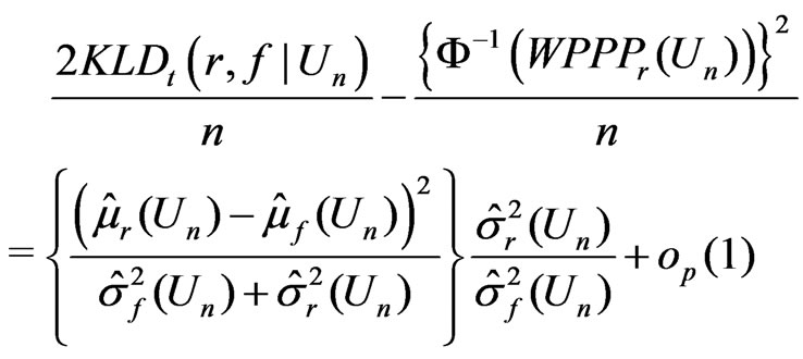
  to be the true model, nor is the true model to be specified. Also, while G-R KLD has been limited to comparing nested generalized linear models, the G-R-A KLD seems to be more flexible for comparing nested or non-nested models that are broader than generalized linear models (see Sections 3 and 4). Theorem 1 shows that under certain regularity conditions, the asymptotic expression of the posterior estimator of G-R-A KLD is comprised of a leading term for model discrepancy in the mean of
 , a term for model discrepancy in the variance of
 , and a constant to penalize model complexity, plus a smaller order term. Since the first two leading terms in the G-R-A KLD estimator resemble a measure that differentiates the predictability between models
  and
and , it is natural to study its connection with Bayesian model discrepancy measures based on predictive statistics (Guttman [8], Rubin [9], Gelman et al. [10]). In particular, we consider the posterior predictive check technique using a one-sided weighted posterior predictive p-value (WPPP). The WPPP of
  evaluates the predictive distribution of
  under
under  at
at , where
  denotes the prediction of
  under
under , the posteriors are derived under
 , and the weight is used to account for the variation of
  under
under . Theorem 2 explicitly shows that for any
  satisfying certain asymptotic normality and regularity conditions, how the model discrepancy is reflected by the G-R-A KLD in connection to that by WPPP. To verify the results in Theorem 1 and Theorem 2 as well as to evaluate G-R-A KLD under partial violation of the regularity conditions, we examine the (asymptotic) property of G-R-A KLD and WPPP via both simulations and real data applications motivated by two cohort studies of diabetes. These examples include the comparison between nested models as well as non-nested models.
The paper is organized as follows. Section 2 studies the G-R-A KLD for (predictive) p.d.f.s of  between two competing models. It also derives the relationship between G-R-A KLD and WPPP. Sections 3 and 4 evaluate model fit using both G-R-A and WPPP for examples that meet all the regularity conditions required in Theorems 1 and 2 as well as for examples that meet only part of these regularity conditions.
2. A Proposed Kullback-Leibler Divergence
2.1. Notations
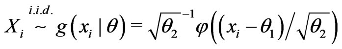
Throughout this paper, we assume that ’s originate from model
 , and are i.i.d. with some common p.d.f. with parameter(s)
  for
for , where
  is a closed set. Denote
  for the reference model and
  for the fitted model, both governed by
 , where
  and
and  are the corresponding the parameter spaces. Also, when a capital letter is used to denote for a random variable (or an estimator), the corresponding lower case is for its realization (or an estimate). Let
 be the base for deriving the posterior density of
  under model
 . We shall denote
  and
and  for the p.d.f.’s of * given
  under model
  and
and , respectively. Also, let
  where
where  is l-dimensional.
2.2. Define Kullback-Leibler Divergence
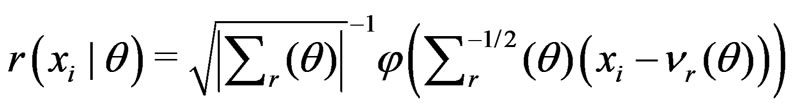
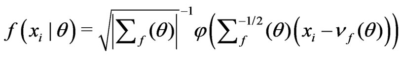
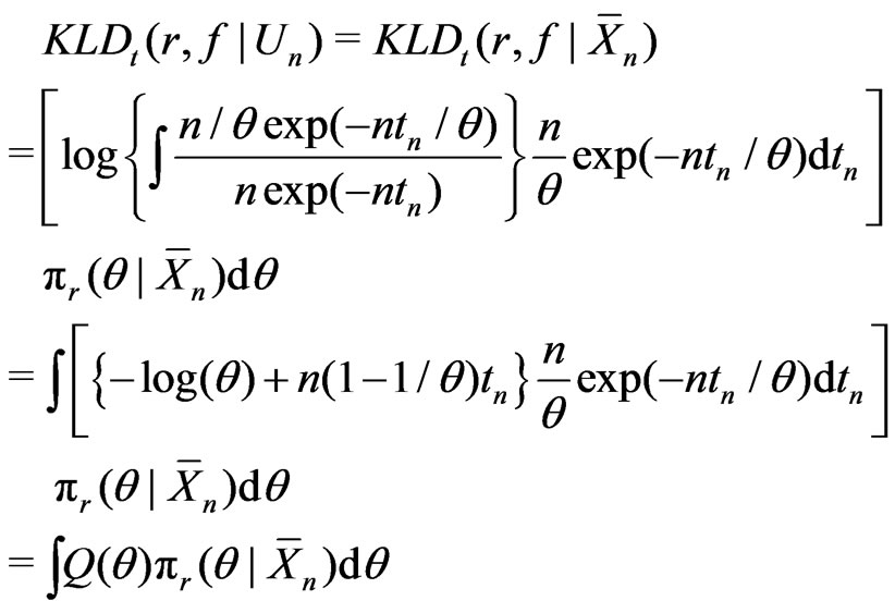
Consider that model adequacy is evaluated based on its fit for certain statistics  that is pertinent to the inference or model diagnostics. Stemmed from Goutis and Robert [1], we assess the relative fit between models using the KLD of the distribution of
  under
under  and that under
  evaluated at
 , the MLE of
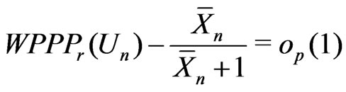
 :
:
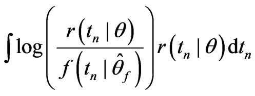 , (1)
, (1)
We shall refer (1) to as the Goutis-Robert-Akaike KLD or G-R-A KLD since (1) is asymptotically equivalent to the KLD proposed by Goutis and Robert [1] when the reference model  is the true model (ref. Akaike [2]).
In general, for each , G-R-A KLD given in (1) can be regarded as a measure of the minimal information gain in model
  from model
  since the minimum information loss under f is achieved at
 . Note that unlike G-R KLD (Goutis and Robert [1]), (1) by definition does not require the reference model
  to be the true model. To understand the utility of (1) in the Bayesian framework, below we derive its Bayesian estimate and the associated (asymptotic) property under certain regularity conditions (see Sections 2.3 and 2.4). We also study the property of (1) when partial regularity conditions hold true using simulated data (Section 3) as well as two applications of diabetes studies (Section 4).
2.3. Bayesian Estimation of the Proposed KLD
Estimating (1) involves approximating the integral with respect to  and estimating unknown model parameters
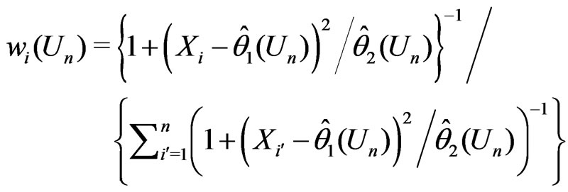
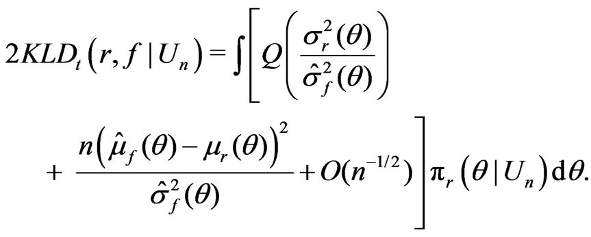
 . To account for the uncertainty of model parameters, we consider the following estimator:
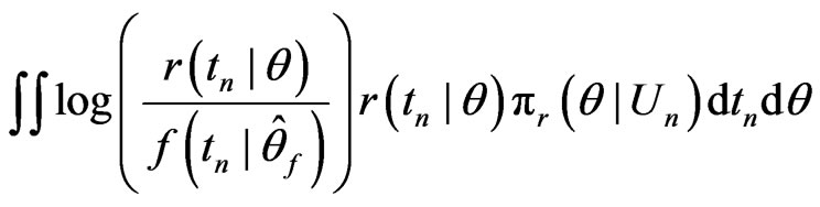 , (2)
, (2)
where , as a function of
 , is used for deriving the posterior of
 , and
, and 
 denoting the posterior density of
  under model
 . That is, (2) is the average discrepancy between
  and
and , each being weighted by
 . We shall denote (2) by
 . Since (2) is nonnegative for any given
 , the closer it is to zero, the less is the information loss by fitting
 , instead of
 , to statistic
 .
.
To gain further insight about the utility of (2), we derive its asymptotic properties below. The approximation of (2) is tied to the assumptions of  under
under  and
and , which will be described in Theorems 1 and 2. In what follows, let the
  statements be interpreted as “almost sure” statements. Also, define
  for
for  which has a unique minimum attained at
 . Denote
  for model parameters, and
 ,
, 
 ,
,  and
and  for the posterior means (or the MLE’s) of
 ,
,  ,
,  , and
, and , respectively.
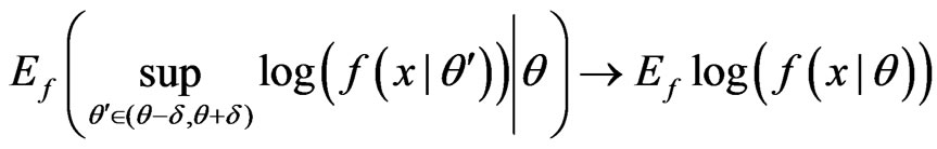
Assume the following regularity conditions under Theorems 1 and 2.
(A1) For each , both
  and
and 
 are 3 times continuously differentiable in
 . Further, there exist neighborhoods
  and
and  of
of  and integrable functions
  and
and  such that
and
for k = 1, 2, 3.
(A2) For all sufficiently large ,
,
and
 .
.
(A3)

as , and
, and
as .
.
(A4) The prior density  is continuously differentiable in a neighborhood of
  and
and .
.
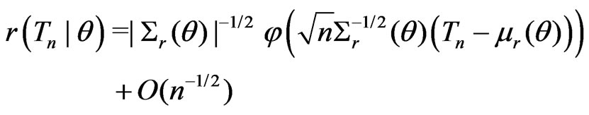
(A5) Let  be asymptotically normally distributed under both models such that
 (3)
(3)
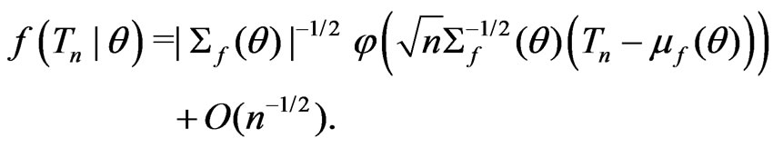
and
 . (4)
. (4)
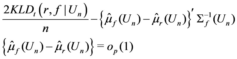
Theorem 1.
 (5)
(5)
when , and
, and
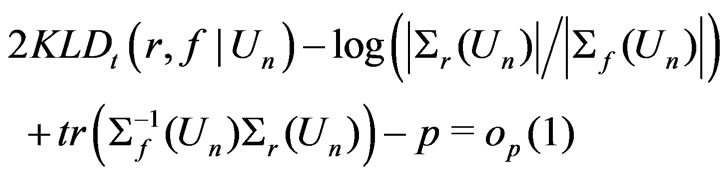
 (6)
(6)
when  but
but .
.
The proof of Theorem 1 is given in Appendix 1. Since model comparison in real applications can rely on the relative fit to a multi-dimensional statistic, it is useful to study whether the results in Theorem 1 are applicable to the multivariate case with a fixed dimension. Suppose that  is a p-dimensional statistic (
 and independent of n) with
and
Then following the derivation given in Appendix 1, it can be shown that
when , and
, and
when  and
and .
.
The result above implies the importance of choosing  to yield an effective model diagnostic based on
 . For example,
  is typically chosen to be the sufficient statistic for
  since it contains all the information of
 . Yet,
  clearly is not the best diagnostic statistic if the estimates of the mean of
  are unbiased under both models
  and
and  as
as
 . Also, note that both
 in (5) and
 in (6) can be viewed as a discrepancy between
  and
and  in terms of their posterior predictivity of
 . We show next how
  is related to a weighted posterior predictive p-value, a typical approach for assessing model discrepancy regarding the predictivity of
  in the Bayesian framework (see Rubin [9]; Gelman et al. [10]).
2.4. KLD vs Posterior Predictive p-Value
Consider
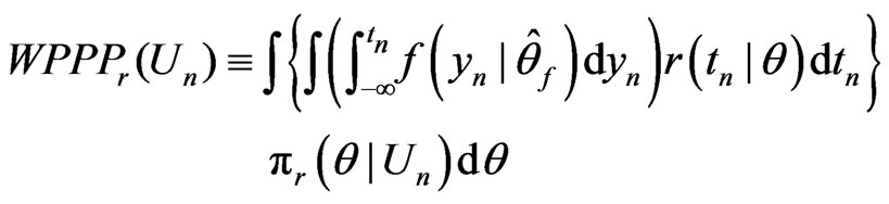 , (7)
, (7)
where  and
and  are the density functions of
  under
under  and
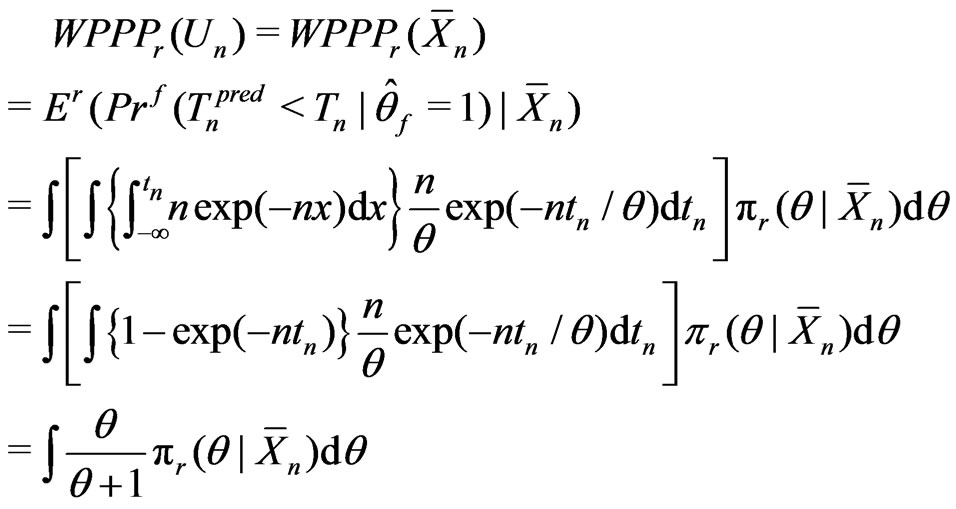
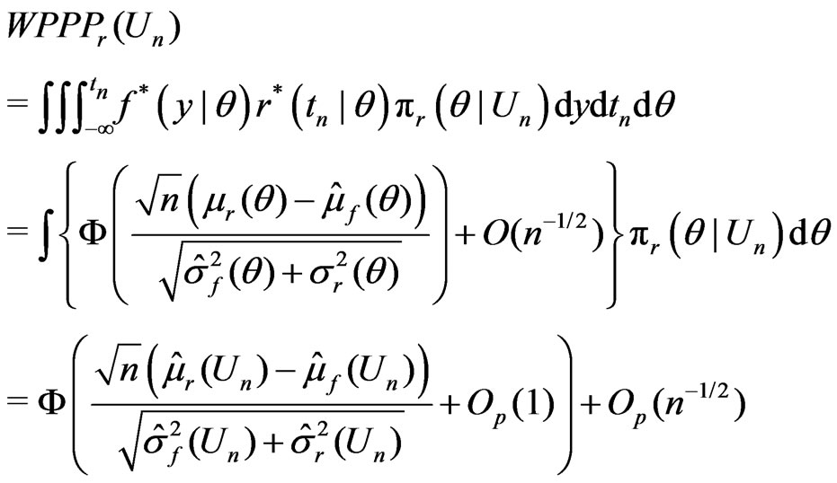
and , respectively. We shall call (7) a onesided weighted posterior predictive p-value (or WPPP) with respect to model
  since as shown above, it is equivalent to the mean predictive p-value of
  under
under  over all possible posterior predicted values of
  arising from
 . Thus WPPP can be viewed as a model discrepancy measure since it evaluates the predictivity of
  under
under . Note that WPPP proposed here differs from the posterior predictive p-value originally proposed in Rubin [9]: WPPP calculates the predictive p-value of
  under an assumed model
  should
  originate from the reference model
 , while Rubin's original proposal [9] assesses the predictive p-value of
  under an assumed model. WPPP is considered here since it is more coherent with the nature of G-R-A KLD as a discrepancy measure between models
  and
and .
.
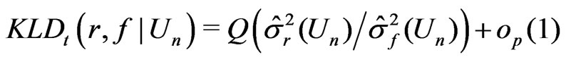
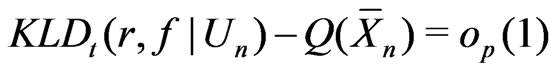
The connection between  and
and 
 is derived in Theorem 2 below. Here we assume regularity conditions (A1)-(A5) as assumed in Theorem 1.
Theorem 2.
 (8)
(8)
when ; and
; and
 (9)
(9)
and
 (10)
(10)
when  but
but .
.
The proof of the theorem is given in Appendix 2.
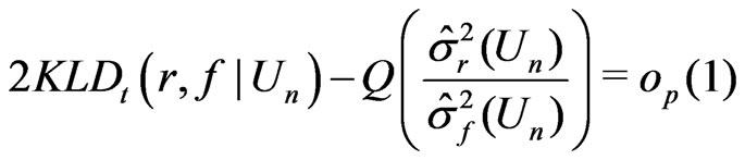
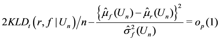
Remark. Theorem 2 explicitly shows the asymptotic relationship between  and
and . Suppose that
  (i.e., the estimate of the mean of
  differs between
  and
and ). Then both
  and
and  are of order
 . Suppose
  but
but  (i.e., the mean of
  is the same both
  and
and , but the variance of
  differs between
  and
and ). Then
  converges to 0, while
 converges to a positive quantity of
 .
.
3. Illustrative Examples
This section demonstrates the utility of the 
 discussed previously through two sets of examples. Examples 3.1-3.6 demonstrate simulated examples that confirm the results proved in Theorems 1 and 2. All these six examples meet the regularity conditions required, while Examples 3.3, 3.5, and 3.6 involve comparing non-nested models. Example 3.7 studies the departure from Theorems 1 and 2 due to violation of the regularity condition (A5). We let
  in all calculations below.
Example 3.1. (Nested) Assume
 where
where . Let
. Let . Suppose that
  and
and
for some known . Then
 ,
,  ,
,  ,
, 
 and
and
 .
.
That is,  converges in probability to a positive quantity, which suggests the discrepancy between
  and
and . However the magnitude of the model discrepancy assessed by
  depends on
 . In contrast,
  converges to 0.5, indicating no difference between
  and
and . Thus the results are consistent with Theorems 1 and 2.
Example 3.2. (Nested) Assume
 where
where 
 ,
,  , and
, and
 is a 2 × 2 matrix with
  and
and
 . Suppose that
and
 where
where ,
,  , and both
 and
and  are 2 × 2 matrices with
 ,
,  ,
,
 , and
, and .
.
Let . Then
 ,
,  and
and .
.
It can be shown that ,
,  ,
,
 and
and
 where
where
 ,
,  ,
, .
.
Thus
 .
.
Since  and
and , following the arguments given in Appendix 2, we have
 Thus both
  and the square of the probit transformed
  suggest the discrepancy between
  and
and  by an
by an  term.
term.
Example 3.3 (Non-nested). Assume
 where
where . Let
. Let ,
,  , and
, and . Then
 ,
,  , and
, and .
.
In this case,  has the same statistical meaning under both
  and
and  since
since . Yet the substantive meaning of
  under
under  differs from that under
 . It can be shown that
 , and
, and
for . Consistent with Theorem 2,
converges in probability to a positive quantity (i.e., ), and
  converges in probability to 0.5 (since
 ).
).
Examples 3.4-3.6 below consider situations where  is an unbiased estimate for the parameter of interest under both
  and
and . However
  is the MLE of certain parameter under
  but not under
 . In these examples, since MLEs of the mean of
  under both
  and
and  converge to the same in probability,
 is reduced to
 in these examples.
Example 3.4 (Nested). As an extension of Example 3.1, consider
 where
where ,
,  ,
,  for
for 
 ,
,  with
with . Let
. Let
 ,
,  and
and
for some . Thus
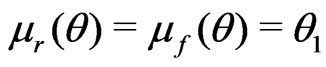 ,
,
 and
and 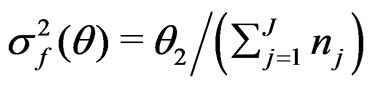 for
for where
where 
 . Here
  is the MLE of
under , while the MLE of
  under
under  is
is
where  is the MLE of
  under
under . Also,
 .
.
We conduct numerical calculation for the following combination ,
,  with
with 
 and
and . Since the 95% percentiles of
  do not exceed 1 under all situations (hence
 , it implies that in the ory KLD should be able to distinguish
  from
from . However, the numerical values of KLD only deviate from 0 by
  for
for 
 . Thus in practice, KLD can hardly be differentiated from
  which converges to 0.5 in probability
 .
.
Example 3.5 (Non-nested). Assume

where . Let
. Let . Suppose that
  are fitted by
  and
and . Then
 ,
,  and
and . Since
for all  with
with  converging to 0 with probability 1 if and only if
 ,
,  can detect model discrepancy in the dispersion parameter. In contrast,
  converges to 0.5 in probability, which is not sensitive to the discrepancy in the dispersion parameter.
Example 3.6 (Non-nested). Assume
where ,
,  , and
, and . Suppose that the empirical variance of
  is greater than 1. Consider fitting the data by
or
 where
where . Let
. Let . Then
  and
and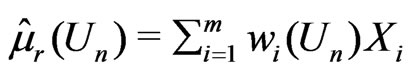 , where
Since both  and
and  are unbiased estimators for
  and
and  converges to 0 in probability,
 where
where , while
  can not be obtained in a closed form. Thus
  is evaluated numerically using eight combinations given in the table below. The results suggest that the degree to which
  can distinguish
  from
from  varies by situation: closer
  and
and  are to 0, closer is
  to 0. In contrast,
  converges to 0.5 in probability, (see Table 1).
Example 3.7 below shows that the asymptotic relationship between  and
and  does not hold in the sense of Theorem 2 due to violation of the asymptotic normality assumption specified in (3) a and (4).
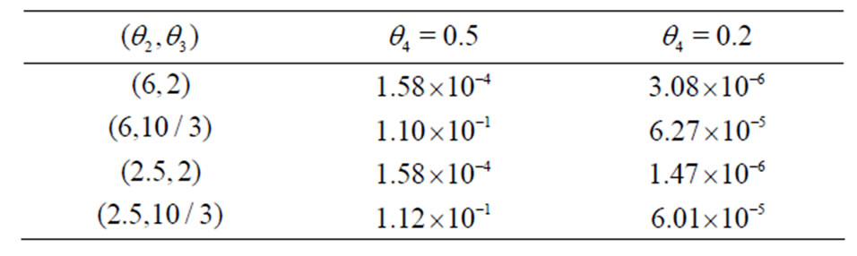
Table 1. Simulation result of example 3.6.
Example 3.7 (Nested). Consider
 .
.
Suppose that  are fitted by
  and
and . Let
. Let . Then
and
 .
.
Then
and
That is,
and
 .
.
In this example, both  and
and 
 can differentiate
  from
from  by an
by an  term despite that the asymptotic relationship between
  and
and  does not hold in the sense of Theorem 2 due to the violation of the asymptotic normality assumption.
4. Application of  to Diabetes Studies
In this section, we apply both  and
and  to compare non-nested models in two studies of diabetes. In these applications, we assess the model fit to the entire dataset due to its clinical implication. Here the selected diagnostic statistic is a multivariate statistic of
  variables, and it does not meet all the regularity conditions specified in Section 3.
4.1. Study I: Analysis of Change in Glucose in Veterans with Type 2 Diabetes
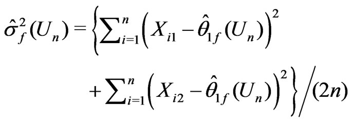
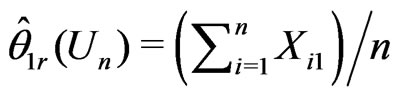
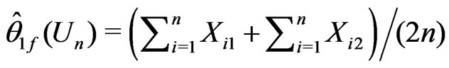
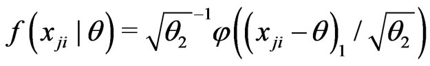
Study I originated from a clinical cohort of 507 veterans with type 2 diabetes who had poor glucose control (indicated by glycosylated hemoglobin A1c or HbA1c greater than 6.5) at the baseline (fiscal year 1999), and were all treated by metformin as the mono oral glucose-lowering agent. As the literature suggested that the glucose-lowering response due to metformin may vary by an individuals obesity status, the goal of our study was to compare models that assessed whether obesity was associated with the net change in glucose level between baseline and the end of 5-year follow-up. In this study, the empirical mean of the net change in HbA1c over the 5 year period was similar between the obese vs. non-obese groups (–0.498 vs. –0.379), yet the empirical variance was greater in the obese group (1.207 vs. 0.865). Also, the distribution of HbA1c was reasonably symmetric. Thus we considered two candidate models for fitting the HbA1c change: a mixture of normals vs. a t-distribution (note that the overall empirical variance of HbA1c change is 1.03); that is,
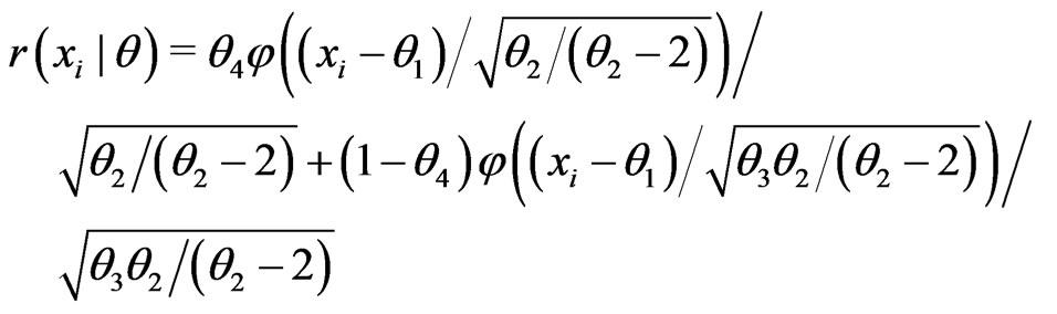
where ,
,  , and
, and  (% in the obesity group) vs.

where . The calculated
  was 5.96, suggesting that model
  provided a modest better fit to the data compared to model
 . This result was also consistent with Figures 1 and 2 which contrasted the empirical quantiles with predicted quantiles under
and . Note that both
  and
and  are unbiased estimators for
 , where
  and
and  with
with

Thus the model discrepancy assessed by 
 is primarily attributed to the difference in the variance assumption between
 and
and (as evident in Figures 1 and 2). In contrast, WPPP = 0.522 suggested that the overall fit were similar between the two models since the estimated net change in HbA1c was similar between these two models.
4.2. Study II: Analysis of the Functioning Score in Older Adults with Diabetes
Study II arose from the subset of 119 participants with diabetes in the San Antonio Longitudinal Study of Aging (SALSA), a community-based study of the disablement process in Mexican American and European American older adults. Details of the SALSA study design, sampling approach, recruitment and field procedures have been described previously (Hazuda et al. [11]). The goal of our analyses was to compare models that assessed whether glucose control trajectory class (poorer vs. better) was associated with the lower-extremity physical functional limitation score during the first follow-up period. The lower-extremity physical functional limitation score was measured by the Short Physical Performance Battery or SPPB, which is a well-established, validated measure of physical functioning. SPPB score is a sum of three items: 8-foot walking times, repeated chair stands, and balance scores, each being a 5-point liker scale 0 - 4. Hence the SPPB score is discrete in nature with a range of 0 - 12. Higher SPPB scores indicate better performance and less functional limitation. Exploratory data analyses suggested that the empirical variance of SPPB (15.60 vs. 14.33) was greater than the mean (7.23 vs. 8.02) in both glucose control classes. Also, due to the

Figure 1. Quantile plot for HbA1c for T2DM participants with obesity in VA (open triangle: quantile estimates based on the model assuming a mixture of normal distributions solid circle: quantile estimates based on the model assuming a t-distribution solid line: empirical quantiles).
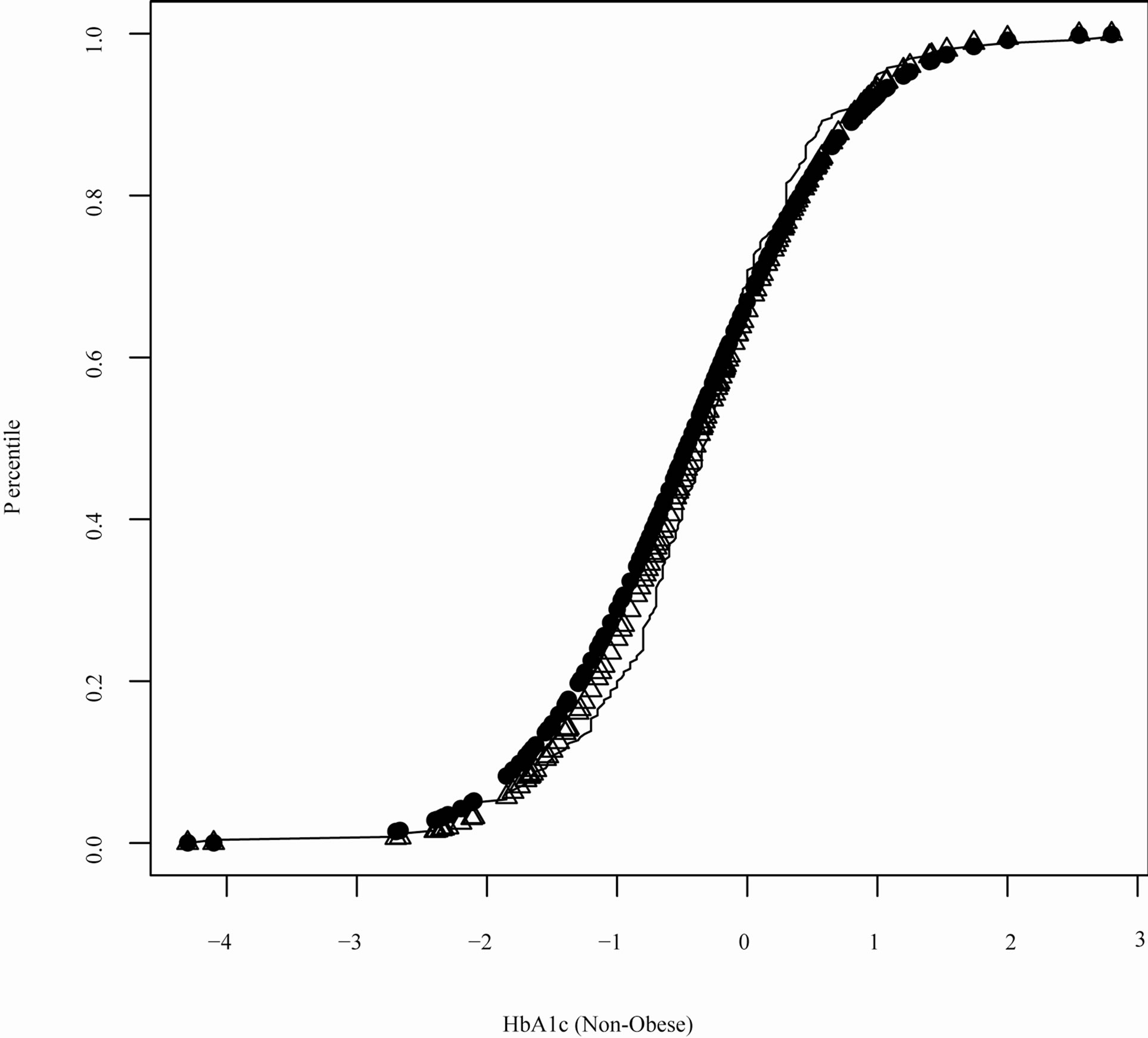
Figure 2. Quantile plot for HbA1c for T2DM participants without obesity in VA (open triangle: quantile estimates based on the model assuming a mixture of normal distributions solid circle: quantile estimates based on the model assuming a t-distribution solid line: empirical quantiles).
left-skewedness of the distribution of SPPB, we considered models fit to the reversed SPPB, i.e.,
 . Given the nature of SPPB distribution, we compare two candidate models:
with  and
and
 .
.
The calculated  is 32.63, suggesting that
  has a much better fit than
 , which is coherent to the quantile plot shown in Figures 3 and 4. Since both
  and
and  yielded similar estimates of
 , the model discrepancy assessed by
  could primarily be attributed to the difference in variance estimation between
  and
and  (as evident in Figure 2). In contrast, WPPP = 0.539 suggested similar fit between
  and
and  as expected due to similar estimates of
  under both
  and
and .
.
5. Discussion
This paper considers the G-R-A KLD as given in (2). This KLD is appropriate for quantifying information discrepancy regarding  contained in the competing models
  and
and . We derive the asymptotic property of the G-R-A KLD in Theorem 1, and its relationship to a weighted posterior predictive p-value (WPPP) in Theo-
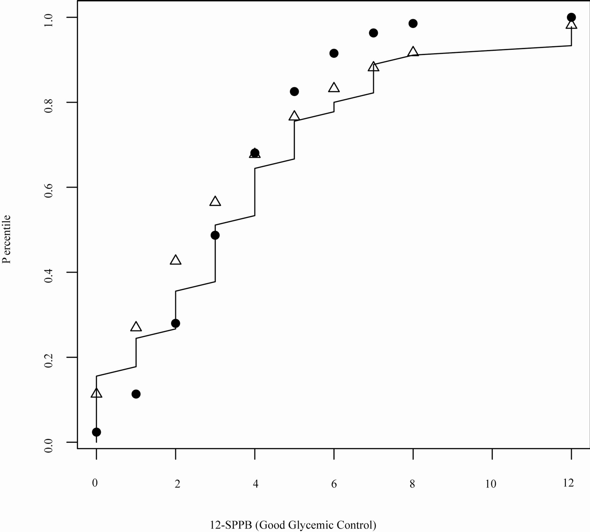
Figure 3. Quantile plot for SPPB for T2DM participants with good glycemic control in SALSA (open triangle: quantile estimates based on the negative binomial model; solid circle: quantile estimates based on the Poisson model; solid line: empirical quantiles).
rem 2. However, our results would need further refinement when the normality assumptions given in (3) and (4) are not suitable (see Example 3.7). As shown in Section 4, model comparison in medical research may rely on the fit to a multidimensional statistic. Although the results in Theorem 1 holds for a multivariate  with a fixed dimension, further investigation is needed to assess the property of our proposed KLD for situations when the dimension of
  increases with
 . The KLD proposed herein usually provides the relative fit between competing models. Thus, for the purpose of assessing model adequacy (rather than relative model fit), a KLD should be used in conjunction with absolute model departure indices such as posterior predictive p-values or residuals. Nevertheless, a KLD can be a measure of the absolute fit of model
  when the superior model
  is the true model, and therefore can be used for checking model adequacy.
6. Acknowledgements
Wang’s research is partially supported by NIDDK K25- DK075092; Ghosh’s research is partially supported by NSF. We thank Dr. Hazuda for providing data from the SALSA study supported by NIA R01-AG10444 and NIA R01-AG16518.
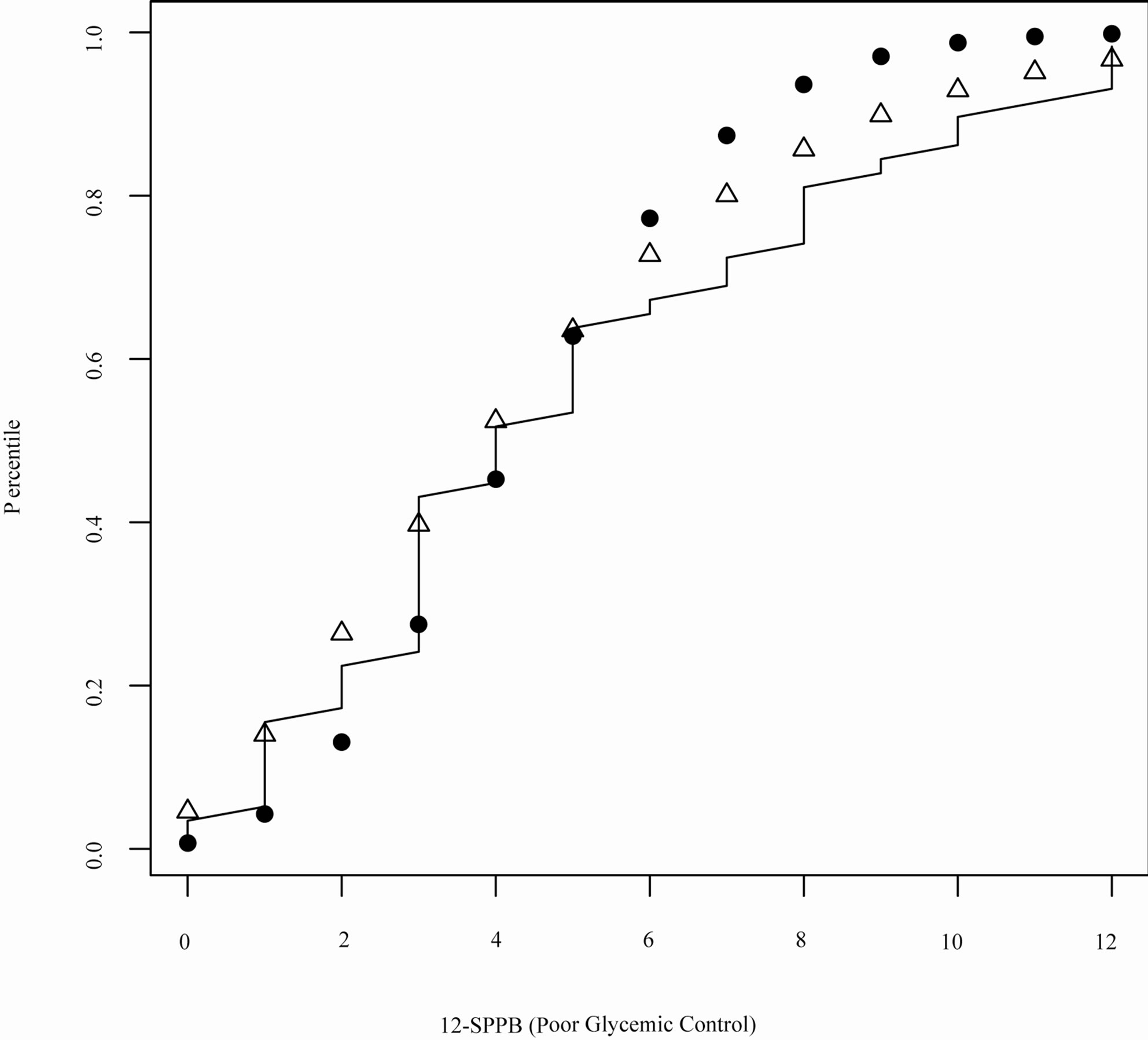
Figure 4. Quantile plot for SPPB for T2DM participants with poor glycemic control in SALSA (open triangle: quantile estimates based on the negative binomial model; solid circle: quantile estimates based on the Poisson model; solid line: empirical quantiles).
7. References
[1] C. Goutis and C. P. Robert, “Model Choice in Generalised Linear Models: A Bayesian Approach via KullbackLeibler Projections,” Biometrika, Vol. 85, No. 1, 1998, pp. 29-37. doi:10.1093/biomet/85.1.29
[2] H. Akiaike, “A New Look at the Statistical Identification Model,” IEEE Transactions on Automatic Control, Vol. 19, No. 6, 1974, pp. 716-723. doi:10.1109/TAC.1974.1100705
[3] C. E. Shannon, “A Mathematical Theory of Communication,” Bell System Technical Journal, Vol. 27, 1948, pp. 379-423 and pp. 623-656.
[4] S. Kullback and R. A. Leibler, “On Information and Sufficiency,” The Annals of Mathematical Statistics, Vol. 22, No. 1, 1951, pp. 79-86. doi:10.1214/aoms/1177729694
[5] D. V. Lindley, “On a Measure of the Information Provided by an Experiment,” The Annals of Mathematical Statistics, Vol. 27, No. 4, 1956, pp. 986-1005. doi:10.1214/aoms/1177728069
[6] J. M. Bernardo, “Expected Information as Expected Utility,” The Annals of Statistics, Vol. 7, No. 3, 1979, pp. 686-690. doi:10.1214/aos/1176344689
[7] G. Schwarz, “Estimating the Dimension of a Model,” The Annals of Statistics, Vol. 6, No. 2, 1978, pp. 461-464. doi:10.1214/aos/1176344136
[8] I. Guttman, “The Use of the Concept of a Future Observation in Goodness-of-Fit Problems,” Journal of the Royal Statistical Society B, Vol. 29, No. 1, 1967, pp. 83-100.
[9] D. B. Rubin, “Bayesianly Justifiable and Relevant Frequency Calculations for the Applies Statistician,” Annals of Statistics, Vol. 12, No. 4, 1984, pp. 1151-1172. doi:10.1214/aos/1176346785
[10] A. Gelman, J. Carlin, H. S. Stern and D. Rubin, “Bayesian Data Analysis,” Chapman and Hall, London, 1996.
[11] H. P. Hazuda, S. M. Haffner, M. P. Stern and C. W. Eifler, “Effects of Acculturation and Socioeconomic Status on Obesity and Diabetes in Mexican Americans: The San Antonio Heart Study,” American Journal of Epidemiology, Vol. 128, No. 6, 1988, pp. 1289-1301.
[12] S. Ghosal and T. Samanta, “Expansion of Bayes Risk for Entropy Loss and Reference Prior in Nonregular Cases,” Statistics and Decisions, Vol. 15, 1997, pp. 129-140.
[13] I. Ibragimov and R. Hasminskii, “Statistical Estimation: Asymptotic Theory,” Springler-Verlag, New York, 1980.
Appendix 1. Proof of Theorem 1
Under (3) and (4), it can be shown that

Applying an argument similar to that in Ghosal and Samanta [12] (see also Ibragimov and Hasminskii [13]), (A1)-(A5) gives
 (11)
(11)
When ,
, 
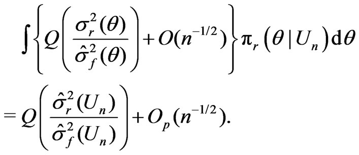
 is the dominating term in (11). Thus by (A1)-(A5) and the arguments similar to those in Ghosal and Samanta [12], one gets
 (12)
(12)
If ,
,  , then (11) becomes
 (13)
(13)
Therefore,
when , and
, and
 .
.
when  and
and .
.
Appendix 2. Proof of Theorem 2
Write  for the realization of
 , a
, a  random variable. Then
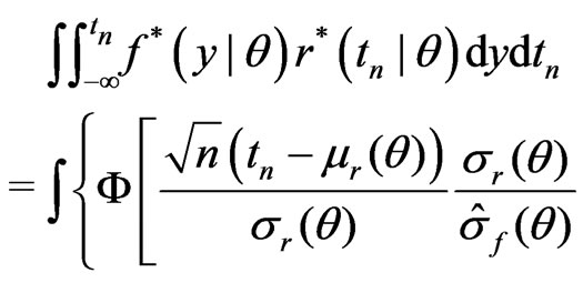
The second equality follows (A1)-(A5) and the argument similar to that used in Ghosal and Samanta [12]. Let  be a
be a  random variable distributed independently of
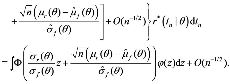
 . Then one can rewrite the above integral as
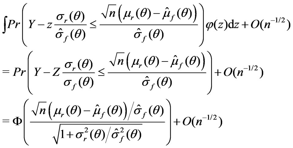

Therefore, applying the arguments similar to those in Ghosal and Samanta [12] under (A1)-(A5) yields
 (14)
(14)
when ; and
; and
 (15)
(15)
when . This completes the proof.