Open Journal of Statistics
Vol.1 No.2(2011), Article ID:6550,6 pages DOI:10.4236/ojs.2011.12010
Sequential Test of Fuzzy Hypotheses
Department of Statistics, Faculty of Sciences, University of Birjand, Southern Khorasan, Iran
E-mail: g_z_akbari@yahoo.com
Received May 22, 2011; revised June 10, 2011; accepted June 17, 2011
Keywords: Canonical Fuzzy Number, Fuzzy Hypotheses, Type I and II Error Sizes, Sequential Probability Ratio Test
Abstract
In testing statistical hypotheses, as in other statistical problems, we may be confronted with fuzzy concepts. This paper deals with the problem of testing hypotheses, when the hypotheses are fuzzy and the data are crisp. We first give new definitions for notion of mass (density) probability function with fuzzy parameter, probability of type I and type II errors and then state and prove the sequential probability ratio test, on the basis of these new errors, for testing fuzzy hypotheses. Numerical examples are also provided to illustrate the approach.
1. Introduction
Statistical analysis, in traditional form, is based on crispness of data, random variable, point estimation, hypotheses, parameter and so on. As there are many different situations in which the above mentioned concepts are imprecise. On the other hand, the theory of fuzzy sets is a well known tool for formulation and analysis of imprecise and subjective concepts. Therefore the sequential probability ratio test with fuzzy hypotheses can be important. The problem of statistical inference in fuzzy environments are developed in different approaches.
Delgado et al. [1] consider the problem of fuzzy hypotheses testing with crisp data. Arnold [2,3] presents an approach to test fuzzily formulated hypotheses, in which he considered fuzzy constraints on the type I and II errors. Holena [4] considers a fuzzy generalization of a sophisticated approach to exploratory data analysis, the general unary hypotheses automaton. Holena [5] presents a principally different approach and motivates by the observational logic and its success in automated knowledge discovery. Neyman-pearson lemma for fuzzy hypotheses testing and Neyman-pearson lemma for fuzzy hypotheses testing with vague data is given by Taheri et al. and Torabi et al. [6,7]. Filzmoser and Viertl [8] present an approach for statistical testing at the basis of fuzzy values by introducing the fuzzy p-value. Some methods of statistical inference with fuzzy data, are reviewed by Viertl [9]. Buckley [10,11] studies the problems of statistical inference in fuzzy environment. Thompson and Geyer [12] proposed the Fuzzy p-values in latent variable problems. Taheri and Arefi [13] exhibit an approach for testing fuzzy hypotheses based on fuzzy test statistics. Parchami et al. [14] consider the problem of testing hypotheses, when the hypotheses are fuzzy and the data are crisp. they first introduce the notion of fuzzy p-value, by applying the extension principle and then present an approach for testing fuzzy hypotheses by comparing a fuzzy p-value and a fuzzy significance level, based on a comparison of two fuzzy sets.
In present work, we first define a new approach for obtaining the probability (density) function, when the random variable is crisp and the parameter of interest is imprecise (fuzzy). Also, the type I and type II errors are introduced based on fuzzy hypotheses. Then, the sequential probability ratio test (SPRT) is defined and extended based on such hypotheses.
We organize the matter in the following way:
In section 2 we describe some basic concepts of fuzzy hypotheses, density (Mass) probability function with fuzzy parameter and necessary definitions. In section 3 we come up sequential probability ratio test based on fuzzy hypotheses. In section 4 the previous definitions and the sequential probability ratio test will be illustrated by examples.
2. Preliminaries
In this section we describe fuzzy hypotheses, density (Mass) probability function with fuzzy parameter and necessary definitions.
Let  be a probability space, a random variable (RV)
  is a measurable function from
  to
to , where
  is the probability measure induced by
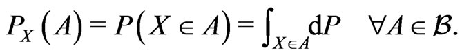
  and is called the distribution of the RV
 , i.e.,
If  is dominated by a
  finite measure
 , i.e.
  then by the Radon-Nikodym theorem (Billingsley, [15]), we have
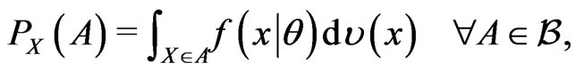
where  is the Radon-Nikodym derivative of
  with respect to
  and is called the probability density function of
  with respect to
 . In a statistical context, the measure
  is usually a “counting measure” or a “Lebesgue measure”, hence
  is
is
 or
or , respectively.
2.1. Canonical Fuzzy Numbers
Let  be the “support” or “sample space” of
 , then a fuzzy subset
  of
of  is defined by its membership function
 . We denote by
  the
the  cut set of
  and
and  is the closure of the set
 , and
, and
1)  is called a normal fuzzy set if there exists
  such that
 ;
;
2)  is called a convex fuzzy set if
  for all
 ;
;
3)  is called a fuzzy number if
  is a normal convex fuzzy set and its
  cut sets, are bounded
 ;
;
4)  is called a closed fuzzy number if
  is a fuzzy number and its membership function
  is upper semicontinuous;
5)  is called a bounded fuzzy number if
  is a fuzzy number and the support of its membership function
  is compact.
If  is a closed and bounded fuzzy number with
  and
and  and its membership function be strictly increasing on the interval
  and strictly decreasing on the interval
  , then
  is called a canonical fuzzy number (Klir and Yuan, [16]).
The fuzzy canonical numbers (such as triangular or trapezoidal fuzzy numbers) are very realistic in fuzzy set theory, so we use this numbers for our goal.
2.2. Fuzzy Hypotheses
We define some models, as fuzzy sets of real numbers, for modeling the extended versions of the simple, the one-sided, and the two-sided ordinary (crisp) hypotheses to the fuzzy ones.
Testing statistical hypothesis is a main branch of statistical inference. Typically, a statistical hypothesis is an assertion about the probability distribution of one or more random variable(s). Traditionally, all statisticians assume the hypothesis for which we wish provide a test are well-defined. This limitation, sometimes, force the statistician to make decision procedure in an unrealistic manner. This is because in realistic problems, we may come across non-precise (fuzzy) hypothesis. For example, suppose that  is the proportion of a population which have a disease. We take a random sample of elements and study the sample for having some idea about
 . In crisp hypothesis testing, one uses the hypotheses of the form:
  versus
  or
or  versus
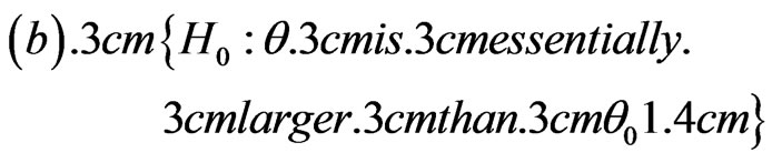
 , and so on. However, we would sometimes like to test more realistic hypotheses. In this example, more realistic expressions about
  would be considered as: “small”, “very small”, “large”, “approximately 0.2”, “essentially larger” and so on. Therefore, more realistic formulation of the hypotheses might be
  is small, versus
  is not small. We call such expressions as fuzzy hypotheses.
We define some models, as fuzzy sets of real numbers, for modeling the extended versions of the simple, the one-sided, and the two-sided crisp hypotheses to the fuzzy ones (Akbari and Rezaei, [17]).
Definition 2.1 Let  be a real number and known.
1) Any hypothesis of the form  is called to be a fuzzy simple hypothesis.
2) Any hypothesis of the form  is called to be a fuzzy two-sided hypothesis.
3) Any hypothesis of the form

 is called to be a fuzzy right one-sided hypothesis.
4) Any hypothesis of the form

 is called to be a fuzzy left one-sided hypothesis.
We denote the above definitions by


2.3. Density (Mass) Probability Function
Let  is a RV and let
 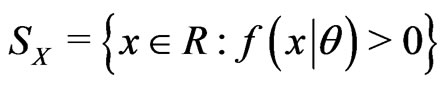 be the “support” or “sample” space of
  and
and
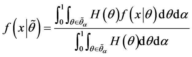
where  is the membership function of canonical fuzzy hypothesis and
  is its
  -cuts.
We call the new density  as the fuzzy probability density (mass) function (FPDF) of
  (Akbari and Rezaei [18]). We note that,
 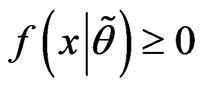 and
and
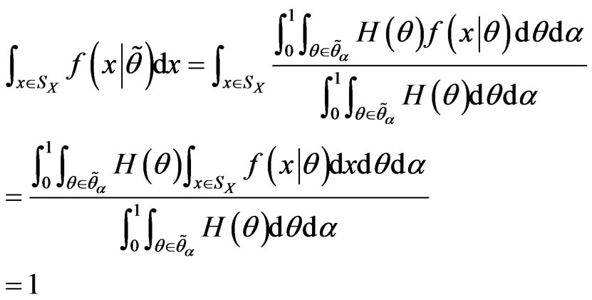
(substitute the summation by integral in discrete cases).
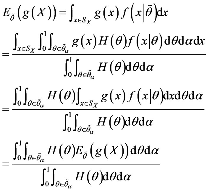
Let 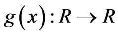 be arbitrary function in
 . Then we define
Let  be a random sample, with observed value
 , where
  has the FPDF
  with unknown
 . For testing
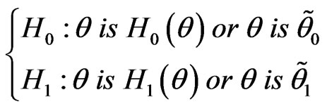
we state the following definitions:
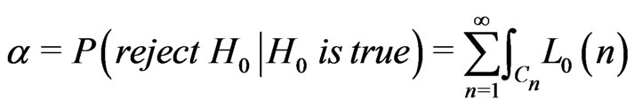
Definition 2.2 Let  be a test function. The probability of type I error of
  is
is
 and the probability of type II error of
  is
is
 .
.
Definition 2.3 A teat  is said to be a test of level
  if
if , where
 .
.
we call  the size of
 .
.
3. Sequential Probability Ratio Test
Consider testing a null fuzzy hypothesis against a alternative fuzzy hypothesis. In other words, suppose a sample can be drawn from one of two FPDFs and it is desired to test that the sample came from one distribution against the possibility that is came from the other. If  denotes the random variables, we want to test
 versus
 . The simple likelihood-ratio test was of the following form:

The sequential test that we propose to consider employs the likelihood-ratios sequentially. Define

for  and compute sequentially
  for fixed
  and
and  satisfying
 , adopt the following procedure: take observation
  and compute
 ; if
; if , reject
 ; if
; if , accept
 ; and if
 , take observation
 , and compute
 . If
. If , reject
 ; if
; if , accept
 ; and if
 , take observation
 , and etc. The idea is to continue sampling as long as
  and stop as soon as
  or
or , rejecting
  if
if  and accepting
  if
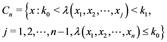
if . The critical region of the described sequential test can be define as
 , where
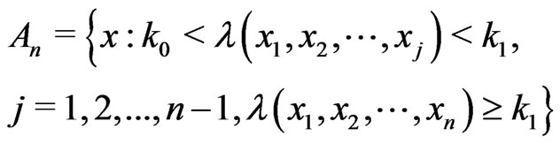
Similarly, the acceptance region can be defined as , where
When we considered the simple likelihood-ratio test for fixed sample size , we determined
  so that the test would have preassigned size
 . We know want to determine
  and
and  so that the sequential probability ratio test will have preassigned
  and
and  for its respective sizes of type I and type II errors. Note that
and

where, as before,  is a shortened notation for
 .
.
For fixed  and
and , the above equations are two equations in the two unknown
  and
and . A solution of these two equations would give the sequential probability ratio test having the desired preassigned error sizes
  and
and . As might be anticipated, the actual determination of
  and
and  from above equations can be a major computational project.
We note that the sample size of a sequential probability ratio test is a random variable. The procedure says to continue sampling until  first falls outside the interval
 . The actual sample size then depend on which
  s observed; it is a function of the random variables
  and consequently is itself a RV. Denote it by
 . Ideally, we would like to know the distribution of
  or at least the expectation of
 . One way of assessing the performance of the sequential probability ratio test would be to evaluate the expected sample size that is required under each hypothesis. The following lemma, given without proof (Lehmann, [20]), state that the sequential probability ratio test with crisp hypotheses is an optimal test if performance is measured using expected sample size. We can similarly prove this lemma with fuzzy hypotheses based on introduced FDPF.
Lemma 3.1 The sequential probability ratio test with error sizes  and
and  minimizes both
  and
and  among all tests which satisfy the following:
 ,
,
 , and the expected sample size is finite.
We noted above that the determination of  and
and  that defines that particular sequential probability ratio test which has error sizes
  and
and  is in general computationally quite difficult. The following lemma (with simple proof) gives an approximation to
  and
and .
.
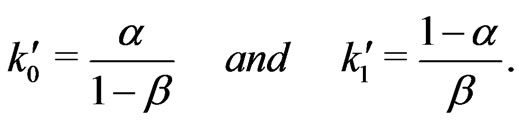
Lemma 3.2 Let  and
and  be defined so that the sequential probability ratio test corresponding to
  and
and  has error sizes
  and
and ; then
  and
and  can be approximated by, say
  and
and , where
Lemma 3.3 Let  and
and  be the error sizes of the sequential probability ratio test defined by
  and
and  given in before lemma. Then
 .
.
Naturally, one would prefer to use that sequential probability ratio test having the desired preassigned error sizes  and
and ; however, since it is difficult to to find the
  and
and  corresponding to such a sequential probability ratio test, instead one can use that sequential probability ratio test defined by
  and
and  of before equation and be assured that the the sum of the error sizes
  and
and  is less than or equal to the sum of the desired error sizes
  and
and .
.
The procedure used in performing a sequential probability ratio test is to continue sampling as long as  and stop sampling as soon as
  or
or
 . If
. If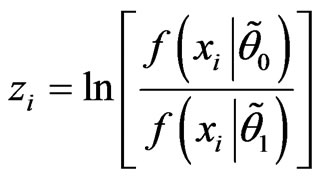 , an equivalent test is given by the following: continue sampling as long as
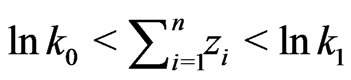 , and stop sampling as soon as
  or
or . As before, let
  be a RV denoting the sample size of the sequential probability ratio test, and let
 .
.
If the sequential probability ratio test leads to rejection of , then the RV
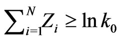 , but
, but  is close to
  since
since  first became less than or equal to
  at the
  th observation; hence
 . Similarly
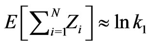 ; hence
 , where
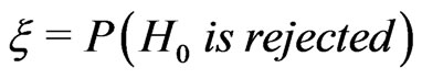 . Using Wald
 s equation (Casella and Berger, [19])
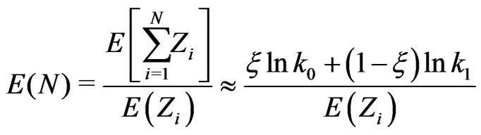
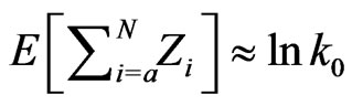
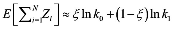
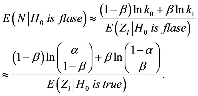
we obtain
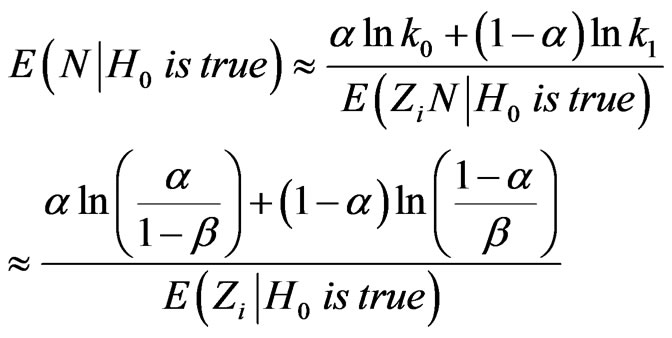
and
4. Numerical Examples
In this section, we illustrate the proposed approach for some distributions and use the ability of package “Maple 6” [21] for this examples.
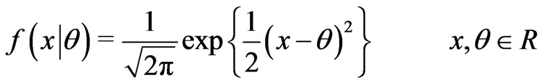
Example 4.1 (Taheri and Behboodian, [6]) Let  be a continues r.v. with PDF

we want to test
where the membership functions  and
and  are defined in the following way:
We can interpret  and
and  as the value of
“ ” and “
 ”.
”.
Let  and
and . We obtain
 ,
, . Hence,
 , and we must take
 whereas
 , thus we take
 .
.
Example 4.2 Let  be a random sample where
  population, i.e.,
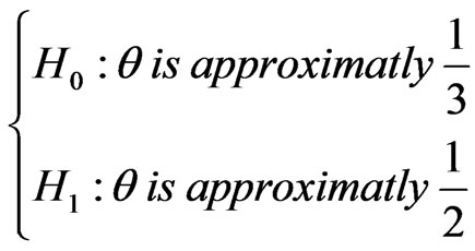
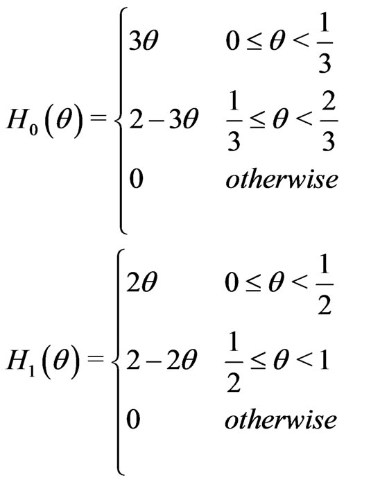
and  s are our fuzzy hypotheses with membership functions given by:
We can interpret  and
and  as the value of “
 ” and “
 ”.
”.
Let . Hence,
 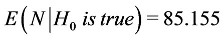 , and we must take
 , whereas
 , thus we take
 .
.
Example 4.3 Let  be a random sample where
  population, i.e.,
and  s are our triangular fuzzy parameters with membership functions

for .
.
We can interpret the canonical parameters as having values that are “near to ”.
”.
Let ,
,  ,
,  and
and . Hence,
 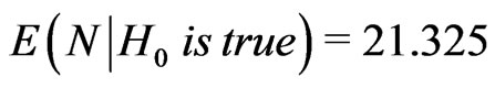 , and we must take
 whereas
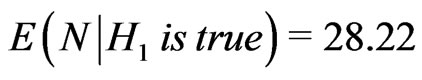 , thus we take
 .
.
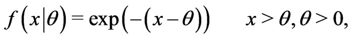
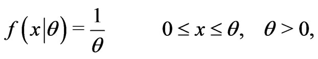
Example 4.4 Let  be a RV from the
  population, i.e.,
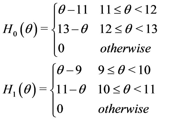
and  s are our trapezoidal fuzzy parameters with membership functions given by:
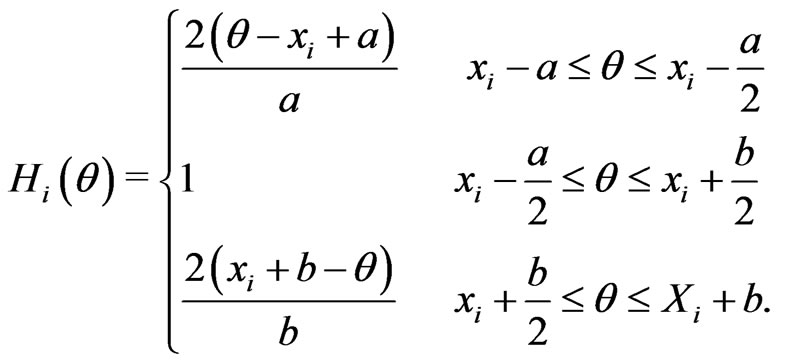
for .
.
Let ,
,  and
and . If
. If , then
 , and we must take
 , whereas
 , thus we take
 .
.
5. Conclusions
In this paper, an new approach for sequential test of fuzzy hypotheses based on fuzzy hypotheses for onesample and two-sample when the available data are crisp, is presented. As for this paper, it sound the introduced method is very simple and applicable in the statistics and other sciences.
Extension of the proposed method to test the variance, correlation and parameters of linear models (regression models), design of experiment is a potential area for the future work. Furthermore, we can construct sequential test of fuzzy hypotheses based on intuitionistic fuzzy hypotheses or fuzzy data for the parameters of interest.
6. References
[1] M. Delgado, J. L. Verdegay and M. A. Vila, “Testing Fuzzy-Hypotheses: A Bayesian Approach,” In: M. M. Gupta, Ed., Approximate Reasoning in Expert Systems, Elsevier Science Ltd, New York, 1995, pp. 307-316.
[2] B. F. Arnold, “An Approach to Fuzzy Hypothesis Testing,” Metrika, Vol. 44, No. 1, 1996, pp. 119-126. doi:10.1007/BF02614060
[3] B. F. Arnold, “Testing Fuzzy Hypothesis with Crisp Data,” Fuzzy Sets and Systems, Vol. 94, No. 3, 1998, pp. 323-333. doi:10.1016/S0165-0114(96)00258-8
[4] M. Holena, “Fuzzy Hypotheses for GUHA Implications,” Fuzzy Sets and Systems, Vol. 98, No. 1, 1998, pp. 101-125. doi:10.1016/S0165-0114(96)00369-7
[5] M. Holena, “Fuzzy Hypotheses Testing in the Framework of Fuzzy Logic,” Fuzzy Sets and Systems, Vol. 145, No. 2, 2004, pp. 229-252. doi:10.1016/S0165-0114(03)00208-2
[6] S. M. Taheri and J. Behboodian, “Neyman-Pearson Lemma for Fuzzy Hypotheses Testing,” Metrika, Vol. 49, No. 1, 1999, pp. 3-17. doi:10.1007/s001840050021
[7] H. Torabi, J. Behboodian and S. M. Taheri, “NeymanPearson Lemma for Fuzzy Hypotheses Testing withVague Data,” Metrika, Vol. 64, No. 3, 2006, pp. 289-304. doi:10.1007/s00184-006-0049-8
[8] P. Filzmoser and R. Viertl, “Testing Hypotheses with Fuzzy Data: The Fuzzy p-value,” Metrika, Vol. 59, No. 1, 2004, pp. 21-29. doi:10.1007/s001840300269
[9] R. Viertl, “Univariate Statistical Analysis with Fuzzy Data,” Computational Statistics and Data Analysis, Vol. 51, No. 1, 2006, pp. 133-147. doi:10.1016/j.csda.2006.04.002
[10] J. J. Buckley, “Fuzzy Probabilities: New Approach and Applications,” Springer-Verlag, Berlin, 2005.
[11] J. J. Buckley, “Fuzzy Probability and Statistics,” Springer -Verlag, Berlin, 2006.
[12] E. A. Thompson and C. J. Geyer, “Fuzzy p-values in Latent Variable Problems,” Biometrika, Vol. 94, No. 1, 2007, pp. 49-60. doi:10.1093/biomet/asm001
[13] S. M. Taheri and M. Arefi, “Testing Fuzzy Hypotheses Based on Fuzzy Statistics,” Soft Computing, Vol. 13, No. 6, 2009, pp. 617-625. doi:10.1007/s00500-008-0339-3
[14] A. Parchami, S. M. Taheri and M. Mashinchi, “Fuzzy p-value in Testing Fuzzy Hypotheses with Crisp Data,” Statistical Papers, Vol. 51, No. 1, 2010, pp. 209-226. doi:10.1007/s00362-008-0133-4
[15] P. Billingsley, “Probability and Measure,” 2nd Edition, John and Wiley, New York, 1995.
[16] G. Klir and B. Yuan, “Fuzzy Sets and Fuzzy Logic-Theory and Applications,” Prentice-Hall, Upper Saddle River, 1995.
[17] M. G. Akbari and A. Rezaei, “Bootstrap Testing Fuzzy Hypotheses and Observations on Fuzzy Statistic,” Expert Systems with Applications, Vol. 37, No. 8, 2010, pp. 5782- 5787. doi:10.1016/j.eswa.2010.02.030
[18] M. G. Akbari and A. Rezaei, “Discrete and Continuous Random Variables with Fuzzy Parameter,” Far East Journal of Theoretical Statistics, Online, 2009.
[19] G. Casella and R. L. Berger, “Statistical Inference,” 2nd Edition, Duxbury Press, Belmont, 2002.
[20] E. L. Lehmann, “Testing Statitical Hypotheses,” Chapman and Hall, London, 1994.
[21] Maple 6, Waterloo Maple Inc. Waterloo, Canada.