Open Journal of Discrete Mathematics
Vol.2 No.2(2012), Article ID:18872,8 pages DOI:10.4236/ojdm.2012.22013
Spline in Compression Methods for Singularly Perturbed 1D Parabolic Equations with Singular Coefficients
1Department of Mathematics, Faculty of Mathematical Sciences, University of Delhi, New Delhi, India
2Department of Mathematics, Deenbandhu Chhotu Ram University of Science & Technology, Murthal, India
3Department of Mathematics, Bharati Vidyapeeth’s College of Engineering, Guru Gobind Singh Indraprastha University, New Delhi, India
Email: *rmohanty@maths.du.ac.in
Received January 16, 2012; revised February 20, 2012; accepted March 11, 2012
Keywords: Spline in Compressions; Parabolic Equations; Two-Level Implicit Schemes; Singular Perturbation; Singular Coefficients; RMS Errors
ABSTRACT
In this article, we discuss three difference schemes; for the numerical solution of singularity perturbed 1-D parabolic equations with singular coefficients using spline in compression. The proposed methods are of  accurate and applicable to problems in both cases singular and non-singular. Stability theory of a proposed method has been discussed and numerical examples have been given in support of the theoretical results.
1. Introduction
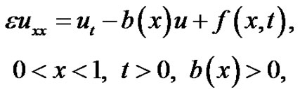
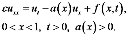
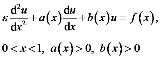
Consider the following singularly perturbed one space dimensional parabolic equation
 (1)
(1)
where and
and 
 for some positive constant K, and
  are continuous bounded functions defined in the semi-infinite region
 .
.
The initial and boundary conditions associated with equation (1) are given by
 (2)
(2)
 (3)
(3)
We assume that the functions, 
 and
and  are sufficiently smooth and their required high-order derivatives exist in the solution space
 .
.
This class of problems arise in various fields of science and engineering, for instance, fluid mechanics, quantum mechanics, optical control, chemical-reactor theory, aerodynamics, geophysics etc. There are a wide variety of asymptotic expansion methods available for solving the problems of the above type. But there can be difficulties in applying these asymptotic expansions in the inner and outer regions, which are not routine exercises but require skill, insight and experimentations. In many applications equation (1) represents boundary or interior layers and has been studied by many authors. Henrici [1] has described the discrete variable methods for ordinary differential equations. Ahlberg et al. [2] and Greville [3] have worked on the theory of splines functions and their applications. An introduction to singular perturbations was given by Malley [4]. Abrahamsson et al. [5] have discussed the finite difference approximations for the system of singularly perturbed ordinary differential equations. Further Prenter [6], Boor [7], and Hemker and Miller [8] have studied various splines and variational methods to solve differential equations. A uniformly accurate difference method for a singular perturbation problem has been analyzed by Berger et al. [9]. Further, Kreiss and Kreiss [10] and Segal [11] have discussed stable numerical methods for singular perturbation problems. Later, Jain and Aziz [12] have derived an efficient numerical method for the solution of convection-diffusion equation using adaptive spline function approximation. Miller et al. [13] have used piecewise uniform meshes for upwind and central difference operators for solving singularly perturbed problems. Kadalbajoo and Patidar [14] have studied the spline in compression methods for the solution of a class of singularly perturbed two point boundary value problems. Later, Mohanty et al. [15] have extended the work discussed in [14] and solved singularly perturbed two point singular boundary value problems. In 2005, Khan and Aziz [16] have discussed the tension spline method for the solution of second order singularly perturbed boundary value problems. Khan et al. [17] have made a survey on various parametric spline function approximations. However, the methods discussed in [17] are only applicable to problems in rectangular coordinates. In the past difficulties were experienced for the numerical solution of singularly perturbed one space dimensional parabolic problems in polar coordinates. The solution usually deteriorates in the vicinity of singularity. In recent past, Mohanty et al. [18] have derived new stable spline in tension methods for singularly perturbed one space dimensional parabolic equations with singular coefficients. In this paper, we have presented a new approach based on spline in compression to solve singularly perturbed parabolic equations of type (1). We have refined our procedure in such a way that the solution retains its order and accuracy even in the vicinity of the singularity x = 0. It is well known that the most classical methods fail when  is small relative to the mesh length h > 0, that is used for discretization of the differential equation (1) in the x-direction. Our aim is to show that compression splines can furnish accurate numerical approximations of equation (1), when all or any of the coefficients
 and
and  contain singularity at x = 0 and when
  is either small or large as compared with h. We consider three types of problems. In the first case, we analyze the problems in which the second derivative term
  and the function term
  are present, whereas the term containing the first term derivative
  is absent. The problems having the second derivative
  term and first derivative term
  but lacking the function term
  are considered in the second case. Finally, the third case deals with the most general problems. In all cases, we use the continuity of first derivative of the spline function. The resulting spline difference methods are two-level implicit schemes (see Figure 1) and of
  accurate and are tridiagonal system of equations at each advanced time level, which can be solved by using a tri-diagonal solver. The main significance of our work is that the proposed compression spline difference schemes are applicable to both singular and non-singular problems. In Section 2, we have discussed the derivation of the spline methods and their application to singular problems. In Section 3, we have discussed stability analysis of a method. In Section 4, numerical results of three different singular problems have been given to demonstrate the utility of the proposed method. The numerical results confirmed that the proposed compression spline methods produce an oscillation-free solution for
  everywhere in the solution region 0 < x < 1, t > 0.
2. Description of the Compression Spline Method
The solution domain  is divided into
  mesh with the spatial step size
  in x-direction and the time step size k > 0 in t-direction respectively, where N and J are positive integers. The mesh ratio parameter is given by
 .
.
Grid points are defined by , l = 0(1) N + 1 and
 . The notations
  and
and  are used for the discrete approximation and the exact solution of
  at the grid point
 , respectively.
Let  and
and 
For , we denote
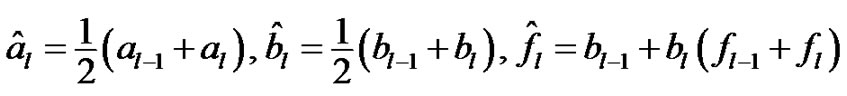 .
.
We consider the following three cases:
Case 1: First we consider the differential equation
 (4)
(4)
which is a particular case of equation (1) in which the first derivative term  is absent.
For the derivation of the method for the equation (4), we follow the approaches given by Kadalbajoo and Patidar [14], and Mohanty et al. [15].
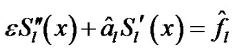
Now we consider the ordinary differential equation
 (5)
(5)
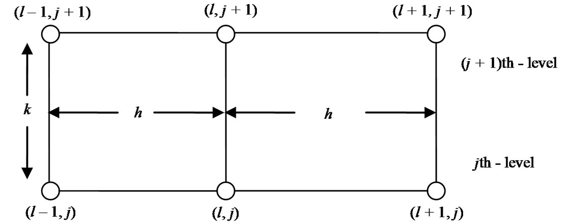
Figure 1. Schematic representation of two-level scheme.
The numerical solution of this equation is sought in the form of the spline function , which on each interval
 , denoted by
  satisfies the differential equation
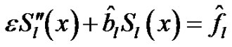 (6)
(6)
The interpolating conditions:
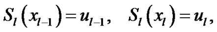 (7)
(7)
and the continuity condition:
 (8)
(8)
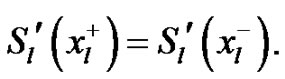
Solving the equation (6) and using the interpolating conditions (7), we get
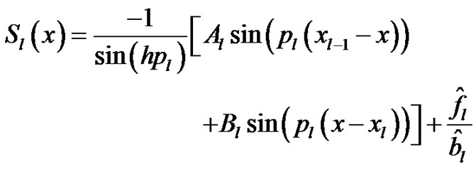 (9)
(9)
if 
where 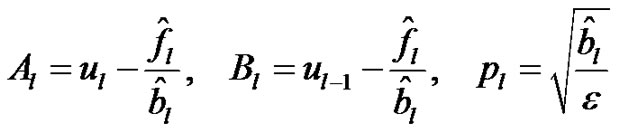
Equation (9) is known as spline in compression, Replacing l by l + 1 in equation (9), we can obtain the spline function  defined in
 .
.
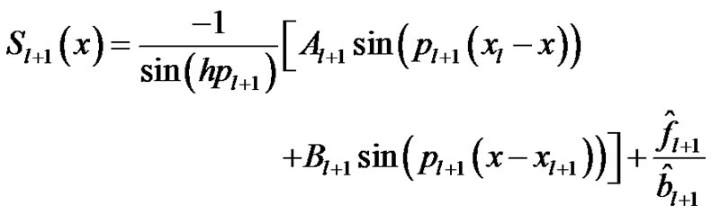 (10)
(10)
Differentiating equation (9) with respect to “x” and using the continuity condition (8), we obtain the spline in compression scheme for the numerical solution of equation (5) as:
 (11)
(11)
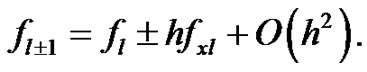
Note that, the scheme (11) is of O(h2) accurate for the numerical solution of (5), however, the scheme fails to compute at l = 1. We overcome this difficulty by using the following approximations:
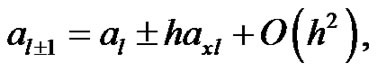 (12a)
(12a)
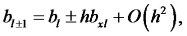 (12b)
(12b)
 (12c)
(12c)
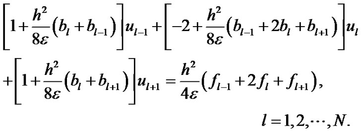
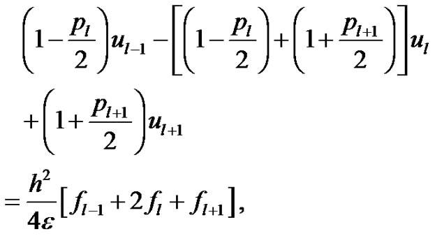
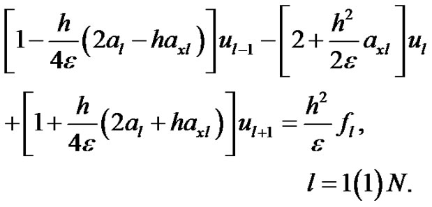
Now using the approximations (12a)-(12c) in equation (11) and neglecting high order terms we obtain the compression spline scheme for the equation (5) in compact form:
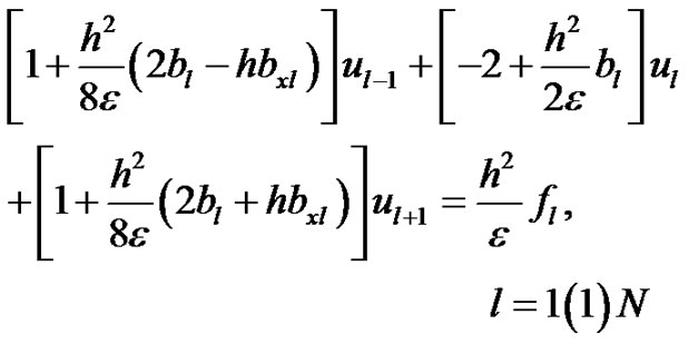 (13)
(13)
In order to obtain the compression spline scheme for the parabolic equation (4), we replace  by
by 
 by
by , and
, and  by
by  [where
 , and
, and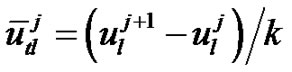 ] in (13) and we obtain
 (14)
(14)
Case 2: In this case, we consider the differential equation of the form
 (15)
(15)
This is a particular case of equation (1), in which the function term  is absent.
For the derivation of the method, we follow the same ideas given by Kadalbajoo and Patidar [14], and Mohanty et al. [15].
We consider the ordinary differential equation
 (16)
(16)
which is a steady-state case of equation (15). As in case 1, we seek S(x) as a solution of the above differential equation
 (17)
(17)
This satisfies the interpolating conditions (7) and the continuity condition (8).
Solving the equation (16) by the help of conditions (7), we obtain
 (18)
(18)
where ,
,  and
and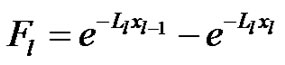 .
.
Similarly, replacing l by l + 1 in equation (18), we can get the spline function  valid in
 .
.
 (19)
(19)
Differentiating equation (18) with respect to “x” and using the continuity condition (8), we may obtain the spline in compression method for the approximate solution of equation (16) as:
 (20)
(20)
where . Note that, the scheme (20) is of O(h2) accurate for the numerical solution of (16), however, the scheme (20) fails to compute at l = 1. We overcome this difficulty by using the approximations defined by (12) and we obtain
 (21)
(21)
In order to obtain the compression spline method for the parabolic equation (15), we replace  by
by

 by
by  and
and  by
by  [where
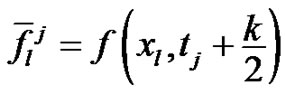 , and
, and ] in (21) and we obtain
 (22)
(22)
Case 3: Finally we consider the most general problem (1), where both  and
and  are present.
For the derivation of the method, we now follow the techniques given by Kadalbajoo and Patidar [14], and Mohanty et al. [15].
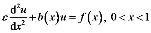
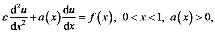
For this purpose, we consider the ordinary differential equation
 (23)
(23)
which is a steady-state case of (1). In this case the spline function  satisfies
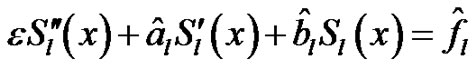 (24)
(24)
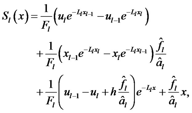
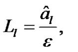
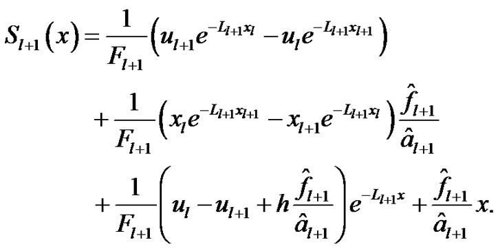
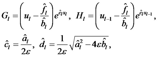
This also satisfies the conditions (7) and (8). Solving the equation (24) with the help of interpolating conditions (7), we obtain
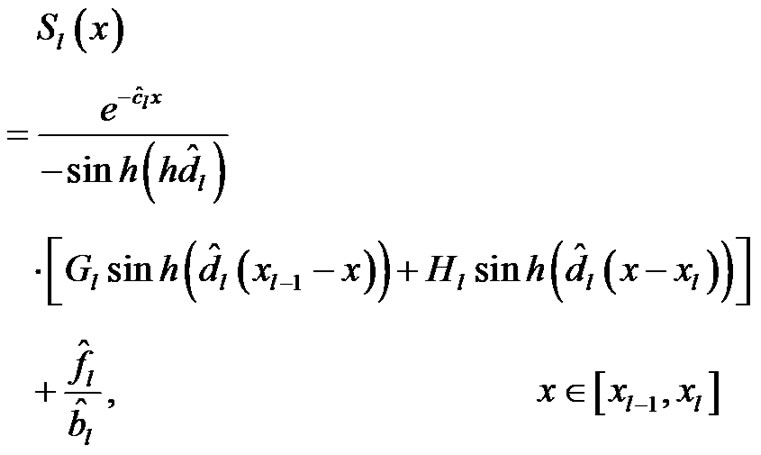
(25)
where
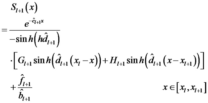
Replacing l by l + 1 in equation (25), we can obtain the spline function  for the equation (24) in the interval
 .
.
Using the continuity condition (8), from equation (25) we obtain the difference scheme based on spline in compression for the approximate solution of equation (23) as
 (27)
(27)
where
 Note that the compression spline scheme (27) is of
  for the approximate solution of the equation (23). However, this scheme fails when the coefficients
 ,
,  and
and  contain singularities and the solution is to be determined at l = 1. We overcome this difficulty by modifying the scheme (27) in such a manner that the solution retains its order and accuracy even in the vicinity of the singularity x = 0.
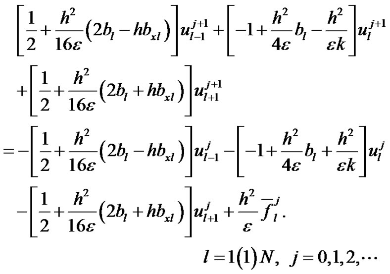
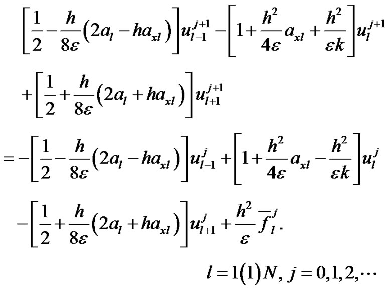
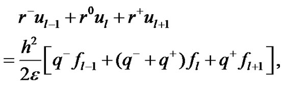
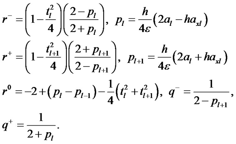
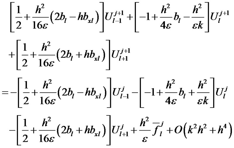
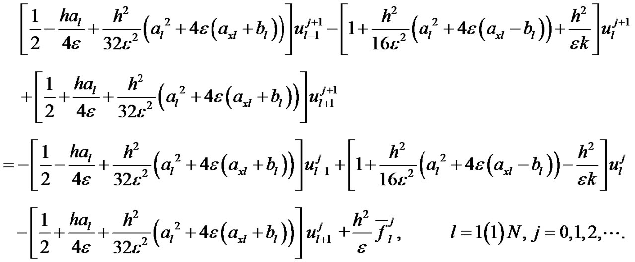
As discussed in case 1 and case 2, using the approximations (12) and neglecting high order terms, we obtain the following compression spline scheme for the solution of parabolic equation (1) in compact form: see (28).
Note that the compression spline schemes (14), (22) and (28) are of  accurate for the numerical solution of singularly perturbed parabolic partial differential equations (4), (15) and (1), respectively and free from the terms
 , hence very easily computed for
 , in the solution region
 .
.
3. Stability Analysis
Now we discuss the stability analysis for the scheme (14).
In this case the exact solution  satisfies
 (29)
(29)
we assume that there exists an error 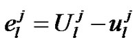 at each grid point (xl, tj), then subtracting (14) from (29), we obtain the error equation
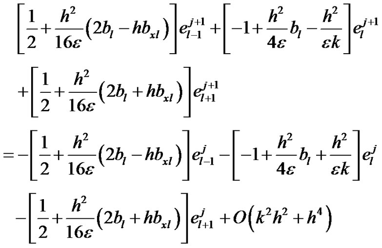 (30)
(30)
To establish stability for the scheme (14), it is necessary to assume that the solution of the homogeneous part of the error Equation (30) is of the form 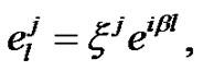 where
where  is in general complex,
  ,
,  is real and we obtain the amplification factor
 (28)
(28)
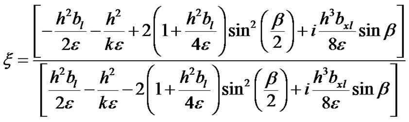
(31)
For stability it is required that . Since
 and
and , it is easy to verify from (31) that
  for all variable angle
 . Hence the scheme (14) is unconditionally stable.
4. Experimental Results
Numerical results presented in this section are concerned with the application of the proposed spline in compression methods to singular perturbation parabolic equations. We have solved the following singularly perturbed singular parabolic equations in the region 0 < x < 1, t > 0 for a fixed value of . The right-hand-side homogeneous functions, initial and boundary conditions may be obtained using the exact solutions as a test procedure. In all cases, we have used Gauss-elimination method (see Saad [19], Hageman and Young [20]) and a tridiagonal solver to solve the problems. All computations were carried out using double length arithmetic.
Example 1:
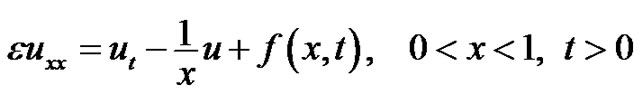 (32)
(32)
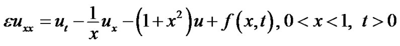
The exact solution is given by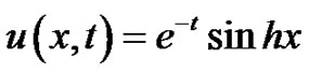 . The root mean square (RMS) errors at t = 0.5 are tabulated in Table 1 for various values of
 .
.
Example 2:
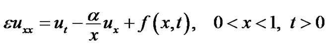 (33)
(33)
The exact solution is given by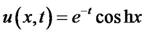 . For
. For  and 2, the equation above represents singularly perturbed linear singular parabolic equation in cylindrical and spherical symmetry, respectively. The RMS errors at t = 1.0 are tabulated in Table 2 for different values of
 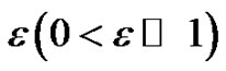 and for
  and 2, respectively.
Example 3:
 (34)
(34)
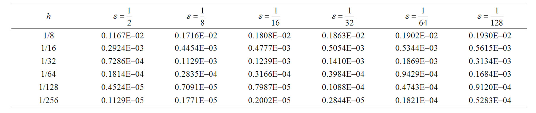
Table 1. The root mean square errors for example 1.
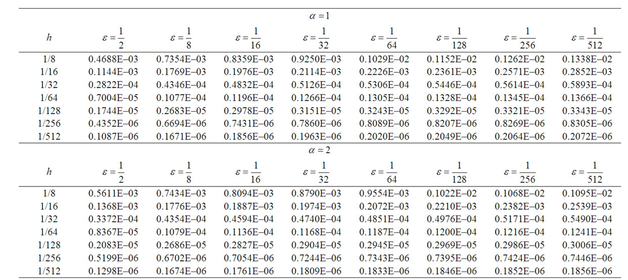
Table 2. The root mean square errors for example 2.
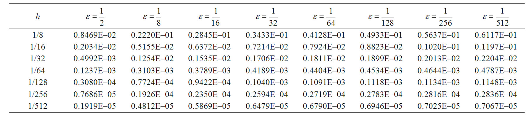
Table 3. The root mean square errors for example 3.
The exact solution is given by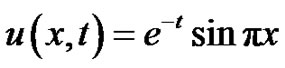 . The RMS errors at t = 1.0 are tabulated in Table 3 for different values of
 .
.
5. Final Discussion
The traditional lower order methods of accuracy of O(k2 + h2) have some inherent difficulties to handle singularly perturbed singular parabolic initial boundary value problems, although some correction techniques may be used to yield stable compression spline methods for . The stability analysis of a compression spline method has been discussed and it has been shown that the method is unconditionally stable. Some text problems have been solved to demonstrate the efficiency of the proposed method when
  is either small or large as compared to the corresponding mesh sizes h > 0 and k > 0. In Table 1, we have reported the RMS errors for the example 1 using the method discussed in case 1. In Table 2, we have given the RMS errors for the singularly perturbed parabolic equation (33) in cylindrical and spherical polar coordinates using the method discussed in case 2. In Table 3, we have tabulated the RMS errors for the more general linear parabolic equation (34) using the method discussed in case 3. All results confirmed that the proposed compression spline methods produce an oscillation-free solution for
  everywhere in the solution region 0< x < 1, t > 0. The technique used in this paper may be extended to derive other numerical methods, not necessarily limited to compression spline methods.
6. Acknowledgements
The authors thank the reviewers for their valuable suggestions, which greatly improved the standard of the paper.
REFERENCES
- P. Henrici, “Discrete Variable Methods in Ordinary Differential Equations,” John Wiley, New York, 1962.
- J. H. Ahlberg, E. N. Nilson and J. H. Walsh, “The Theory of Splines and Their Applications,” Academic Press, New York, 1967.
- T. N. E. Greville, “Theory and Applications of Spline Functions,” Academic Press, New York, 1969.
- R. E. O’Malley, “Introduction to Singular Perturbations,” Academic Press, New York, 1974.
- L. R. Abrahamsson, H. B. Keller and H. O. Kreiss, “Difference Approximations for Singular Perturbations of System of Ordinary Differential Equations,” Numerische Mathematik, Vol. 22, No. 5, 1974, pp. 367-391. doi:10.1007/BF01436920
- P. M. Prenter, “Splines and Variational Methods,” John Wiley, New York, 1975.
- C. de Boor, “A Practical Guide to Splines, Applied Mathematical Science Series 27,” Springer-Verlag, New York, 1978.
- P. W. Hemker and J. J. H. Miller, “Numerical Analysis of Singular Perturbation Problems,” Academic Press, New York, 1979.
- A. Berger, J. M. Solomon and M. Ciment, “An Analysis of a Uniformly Accurate Difference Method for a Singular Perturbation Problem,” Mathematics of Computation, Vol. 37, No. 155, 1981, pp. 79-94. doi:10.1090/S0025-5718-1981-0616361-0
- B. Kreiss and H. O. Kreiss, “Numerical Methods for Singular Perturbation Problems,” SIAM Journal on Numerical Analysis, Vol. 18, No. 2, 1981, pp. 262-276. doi:10.1137/0718019
- A. Segal, “Aspects of Numerical Methods for Elliptic Singular Perturbation Problems,” SIAM Journal on Scientific and Statistical Computing, Vol. 3, No. 3, 1982, pp. 327-349. doi:10.1137/0903020
- M. K. Jain and T. Aziz, “Numerical Solution of Stiff and Convection-Diffusion Equations Using Adaptive Spline Function Approximation,” Applied Mathematical Modelling, Vol. 7, No. 1, 1983, pp. 57-62. doi:10.1016/0307-904X(83)90163-4
- J. J. H. Miller, E. O’Riordan and G. I. Shishkin, “On Piecewise Uniform Meshes for Upwind and Central Difference Operators for Solving Singularly Perturbed Problems,” IMA Journal of Numerical Analysis, Vol. 15, No. 1, 1995, pp. 89-99. doi:10.1093/imanum/15.1.89
- M. K. Kadalbajoo and K. C. Patidar, “Numerical Solution of Singularly Perturbed Two Point Boundary Value Problems by Spline in Compression,” International Journal of Computer Mathematics, Vol. 77, No. 2, 2001, pp. 263-284. doi:10.1080/00207160108805064
- R. K. Mohanty, N. Jha and D. J. Evans, “Spline in Compression Methods for the Numerical Solution of Singularly Perturbed Two Point Singular Boundary Value Problems,” International Journal of Computer Mathematics, Vol. 81, No. 5, 2004, pp. 615-627. doi:10.1080/00207160410001684307
- I. Khan and T. Aziz, “Tension Spline Method for Second Order Singularly Perturbed Boundary Value Problems,” International Journal of Computer Mathematics, Vol. 82, No. 12, 2005, pp. 1547-1553. doi:10.1080/00207160410001684280
- A. Khan, I. Khan and T. Aziz, “A Survey on Parametric Spline Function Approximation,” Applied Mathematics and Computation, Vol. 171, No. 2, 2005, pp. 983-1003. doi:10.1016/j.amc.2005.01.112
- R. K. Mohanty, R. Kumar and V. Dahiya, “Spline in Tension Methods for Singularly Perturbed One Space Dimensional Parabolic Equations with Singular Coefficients,” Neural Parallel & Scientific Computations, Vol. 20, No. 1, 2012, pp. 81-92.
- Y. Saad, “Iterative Methods for Sparse Linear Systems,” SIAM Publication, Philadelphia, 2003.
- L. A. Hageman and D. M. Young, “Applied Iterative Methods,” Dover Publication, New York, 2004.
NOTES
*Corresponding author.