Geomaterials
Vol.3 No.4(2013), Article ID:38557,9 pages DOI:10.4236/gm.2013.34020
Facies and Fracture Network Modeling by a Novel Image Processing Based Method
PETROPARS Ltd. Oil and Gas Developer, Tehran, Iran
Email: Moradi.Pe@ppars.com
Copyright © 2013 Peyman Mohammadmoradi. This is an open access article distributed under the Creative Commons Attribution License, which permits unrestricted use, distribution, and reproduction in any medium, provided the original work is properly cited.
Received March 6, 2013; revised April 6, 2013; accepted April 13, 2013
Keywords: Filter-Based; Image Processing; Pattern; Training Image; Entropy Plot; MPS
ABSTRACT
A wide range of methods for geological reservoir modeling has been offered from which a few can reproduce complex geological settings, especially different facies and fracture networks. Multi Point Statistic (MPS) algorithms by applying image processing techniques and Artificial Intelligence (AI) concepts proved successful to model high-order relations from a visually and statistically explicit model, a training image. In this approach, the patterns of the final image (geological model) are obtained from a training image that defines a conceptual geological scenario for the reservoir by depicting relevant geological patterns expected to be found in the subsurface. The aim is then to reproduce these training patterns within the final image. This work presents a multiple grid filter based MPS algorithm to facies and fracture network images reconstruction. Processor is trained by training images (TIs) which are representative of a spatial phenomenon (fracture network, facies...). Results shown in this paper give visual appealing results for the reconstruction of complex structures. Computationally, it is fast and parsimonious in memory needs.
1. Introduction
Static modeling of complex reservoirs calls for more than two point statistics. Certain features of these objects such as curvilinearity cannot be expressed via two-point relations [1]. Multi Point Statistics (MPS) is used to produce realistic realizations of complex structures after the pioneer work of Strebelle who applied image processing concepts for this purpose [2]. MPS is based on image processing techniques and proposes image construction approach. In this approach, the patterns of the final image to be constructed (facies, fracture network...) are obtained from a training image that depicts relevant geological patterns expected to be found in the subsurface [1]. Furthermore, MPS modeling has the potential to improve estimation in addition to simulation and the so called E-type average value at each node is taken as a local estimated value if training image is appropriate [3].
Training Images (TIs) provide spatial relations, existing patterns and degree of connectivity which must be reproduced in the reconstructed images. The goal is not to reproduce the training image, but to simulate a model that shares some of the multivariate characteristics of the true distribution [4]. To achieve the most appropriate IT, several challenges were raised like: statistical richness of the training image, the scale of the training image, the grid definition of the simulated model, and the univariate distribution of the training image. In this area, Boisvert selects the most data representative TI by comparing the distribution of runs and the multiple point density function from TIs [5]. Boogaart applied variography as an auxiliary element to choose TIs which represent the true joint distribution of the field under consideration [6].
The pattern to point SNESIM method is the first algorithm for MPS modeling [7,8]. SNESIM is a combination of traditional sequential simulation with a search tree concept. Multiple point statistics (observed patterns) of a certain size of training images are stored in a tree structure; Node properties of realizations are then assigned one by one in a search process loop. Search tree is extremely memory demanding. Straubhaar proposed a list of approach modification of SNESIM [9]. Several case studies of successful application of the method are reported [10-14]. Okabe also modified SNESIM for pore network reconstruction [15].
Pattern-to-pattern methods such as SIMPAT [1] FILTERSIM [16] and DisPAT [17] are completely isolated from two-point statistics and eliminate the probabilistic paradigm in MPS algorithms. These methods inherently take the probabilities of the whole multiple point patterns conditioned to the same multiple point data event from the training image [18]. SIMPAT produces visual appealing realizations; however complete search in pattern database is needed. This makes the process of finding the most similar pattern too complex and CPU time-consuming. FILTERSIM reduces pattern dimensions by applying spatial filters and transferring patterns to a lower dimensional space. Coded patterns are then clustered and a prototype is chosen for each bin. This accelerates the search process and decreases run time compared to SIMPAT by means of reducing number of analogy loops. Structures continuity in FILTERSIM method, however, is not preserved as it is in SIMPAT.
Dimensional reduction in patterns is done by applying directional filters [16] or wavelet decomposition on training image [19]. Honarkhah proposed a distance based algorithm DisPAT and automatic information theory based algorithms for selection of optimum template size and dimension of patterns target space [17].
In our previous work [20] one modified FILTERSIM algorithm was proposed for unconditional simulation in which pattern extraction, persisting and pasting steps are modified to enhance visual quality and structures continuity in the realizations. Modifications such as optimum template size selection and additional search steps have considerable improvement in the algorithm performance and produced more visual appealing images compared to FILTERSIM. These changes add marginal computation cost to FILTERSIM because of using pattern frequency concept and yet still much faster than SIMPAT.
In this paper, we propose a novel multiple grid patternto-pattern algorithm for conditional simulation which is a combination of FILTERSIM fastness and SIMPAT accuracy. Results quality and continuity is far better in our proposed algorithm as will be shown shortly.
2. Training Image Processing
Processing of training images consists of gridding, scanning and persisting the corresponding multiple point vectors in a database as shown in Figure 1. Pattern extrac-

Figure 1. Schematic of training image preprocessing steps consist of gridding, scanning and pattern extraction (As template size increases, pattern stores larger scale spatial information).
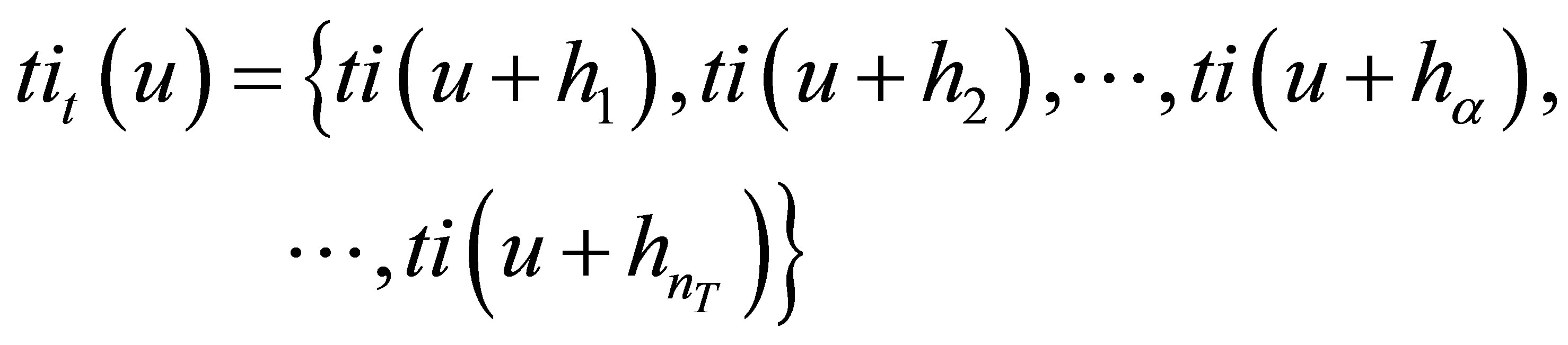
tion can be performed by templates in different sizes. Template size affects the extracted statistics, CPU time and scale of structures in results. A pattern of training image is defined as tit (u) and includes a specific multiple point vector of tit (u) values within a template T centered at node u.
 (1)
(1)
where hα vectors define the geometry of the template nodes;  and nT is the template size. Content of pattern with a frequency component, based on its occurrence frequency in TI, are stored in pattern database patdbT as the following vector:
 (2)
(2)
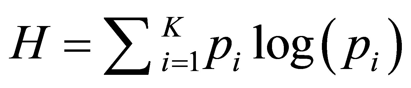
Frequency component of patdbT has the advantage of accelerating selection of appropriate pattern in simulation process. This achieves by elimination of repeated patterns and consequently repeated calculations. Pattern stores larger scale spatial information as the template size increases with the cost of simulation uncertainty and complexity. To find the optimum template size in a single grid simulation, Shannon’s entropy versus template size plot is used [21]. In order to calculate entropy in different template sizes, the following equation is applied:
 (3)
(3)
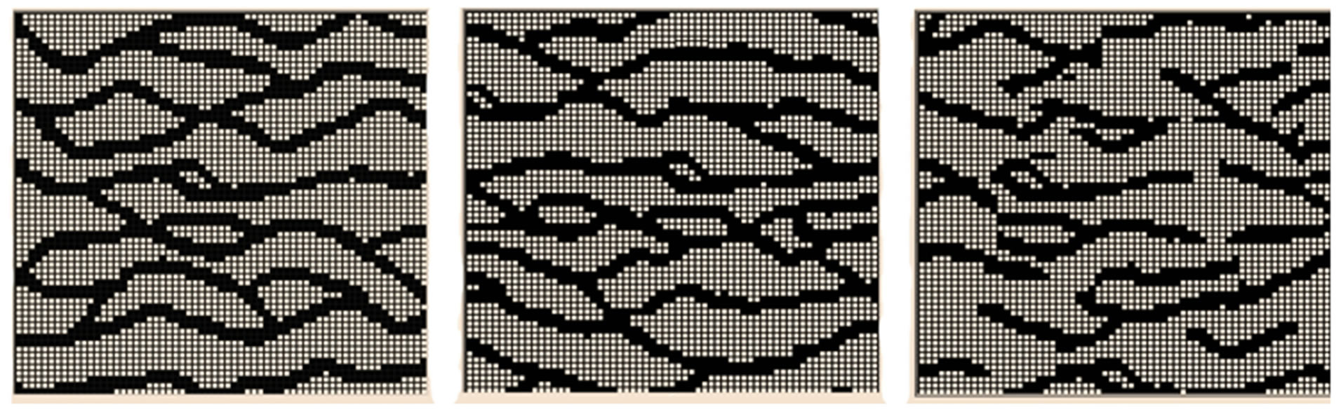
where K = number of possible outcomes of the random variable, and pi represents the probability mass function. Two different behaviors are expected with increasing the template size. In the first stage, entropy will sharply increase since the average number of nodes needed to guess the remaining nodes in the patterns is increased. At a later stage, where the template size has passed the optimal range in an elbow that represents the stationary features of the training image, entropy would increase slowly. This is because the information needed for encoding a large pattern with some stationary features is approximately equal the information of the stationary feature of the training image itself [17]. Mathematical details are discussed extensively by Honarkhah [17]. As shown in results of FILTERSIM automation in Figure 2, spatial statistics of the results are fixed with the passing of the Elbow in entropy plot.
By applying frequency component and optimum template size concepts, training image is scanned with the optimum template size after which the responses of patterns to six directional filters are measured (Table 1). A
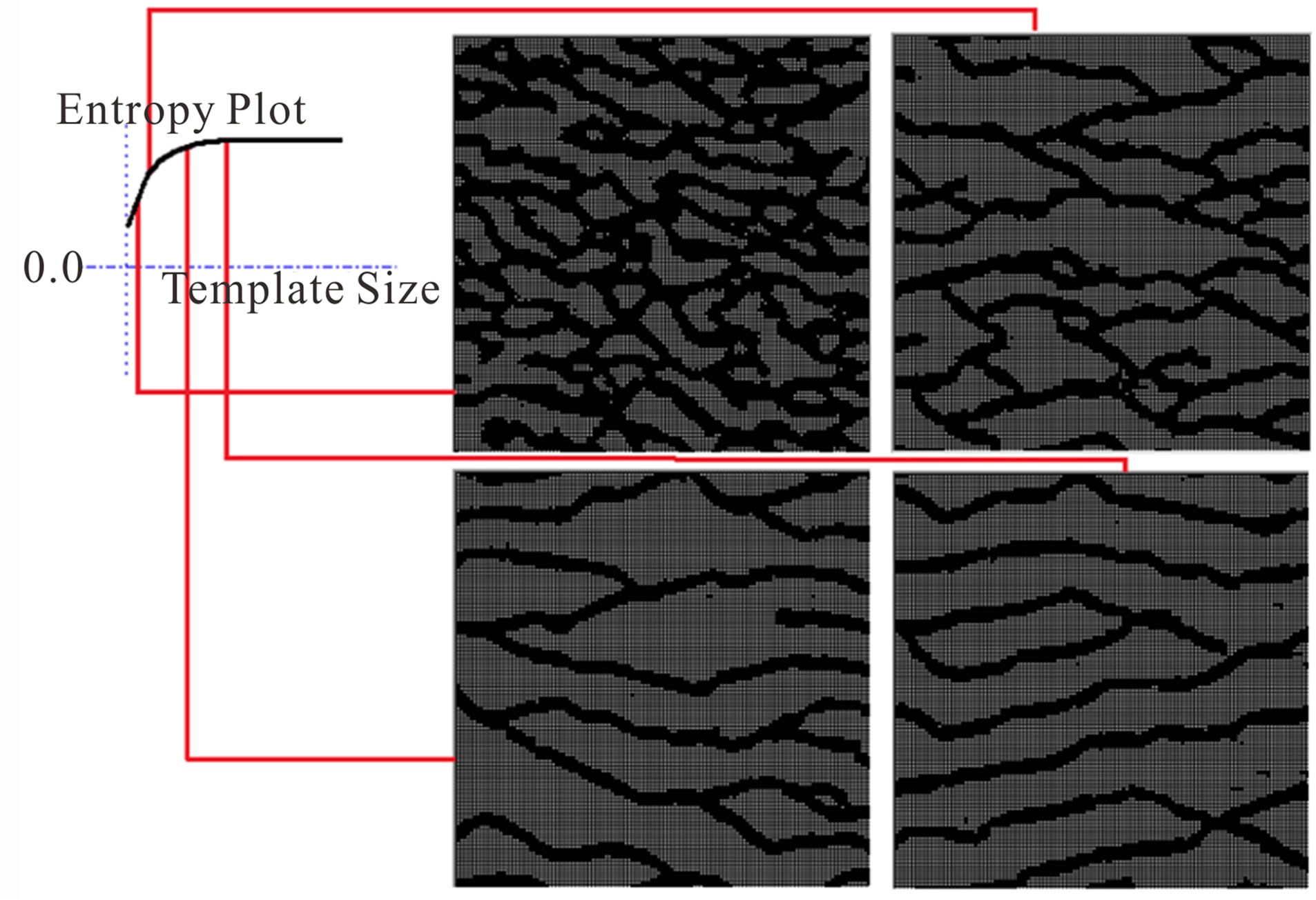
Figure 2. Effect of template size on the simulation results (where the template size has passed the optimal window, stationary features in realizations are approximately equal the information of the stationary feature of the training image).
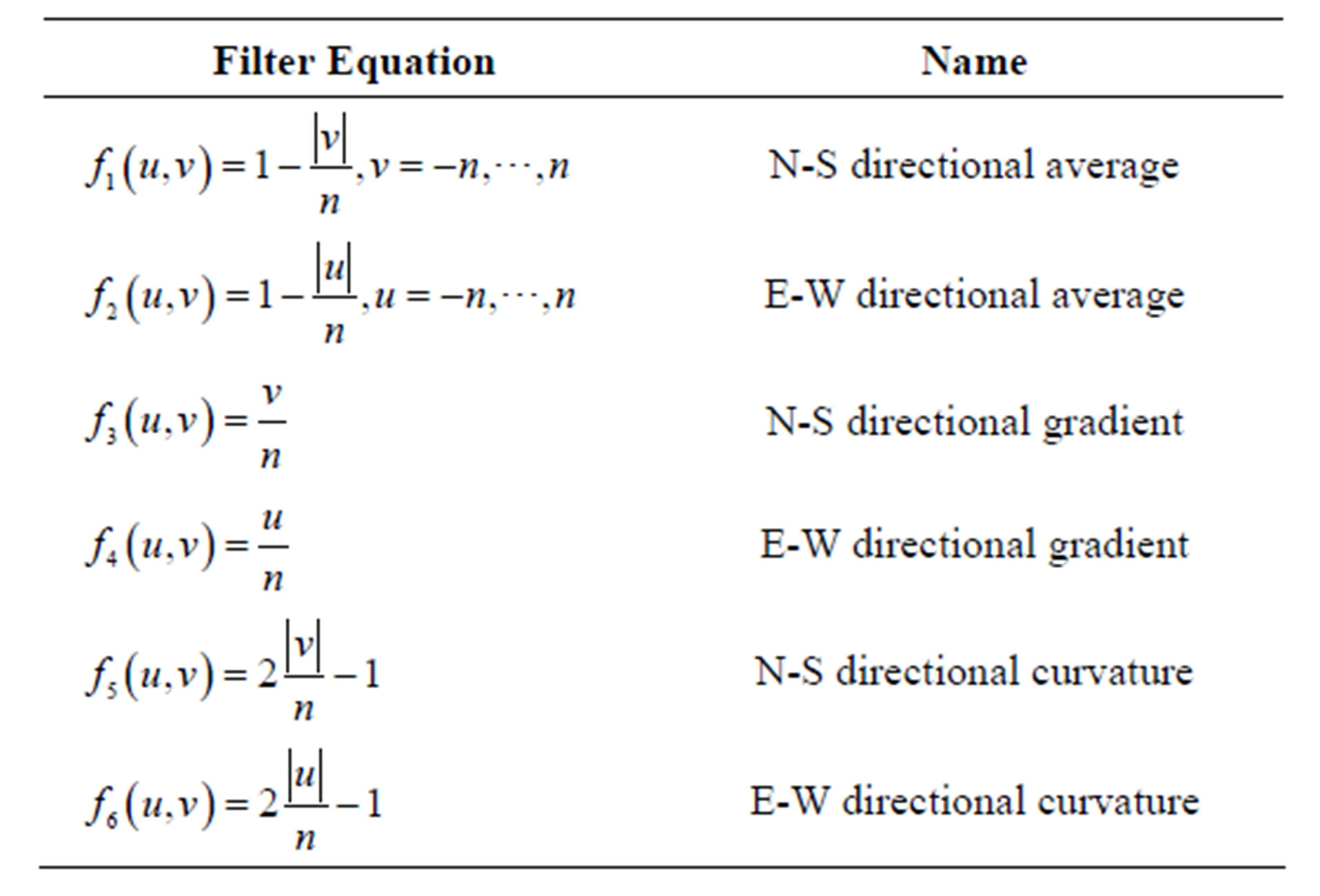
Table 1. Directional filters for dimension reduction of patterns [16].
sample of pattern transferring to a lower dimensional space by measuring the responses of patterns to two directional filters is shown in Figure 3. All extracted patterns are placed with other similar patterns into the specified bins. Figure 4 shows the results of applying this step on the some face pictures.
Each filter score is divided into five categories and cluster the patterns into 5 ^ 6 bins. For each of which one prototype is calculated. Each prototype is binary average of patterns in a specific bin. Many of these created bins are empty and will be eliminated in the search process which is only done on selected prototypes for the filled bins.
Having processed the TI and filled the pattern database as just described, reconstruction of realizations can performed in unconditional and conditional situations. Simulation procedures with and without hard data are discussed in detail in the next sections. Table 2 lists the TI processing steps.
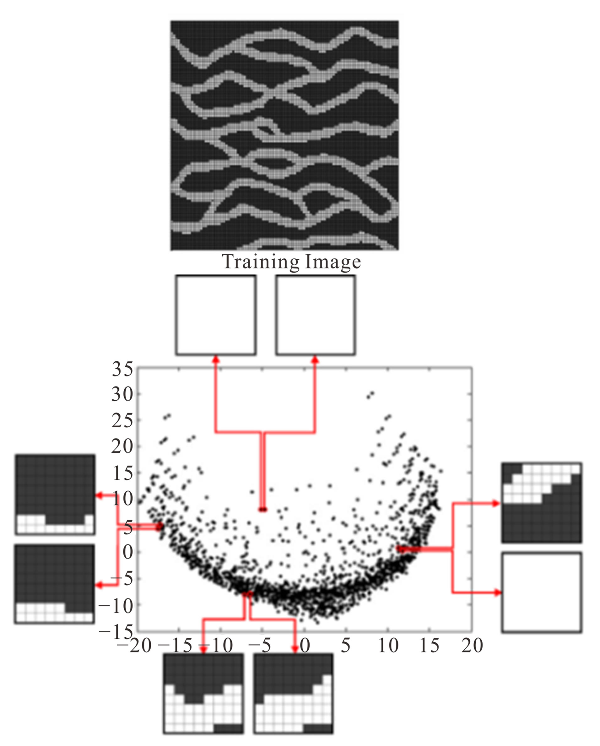
Figure 3. Pattern transferring to a lower dimensional space.
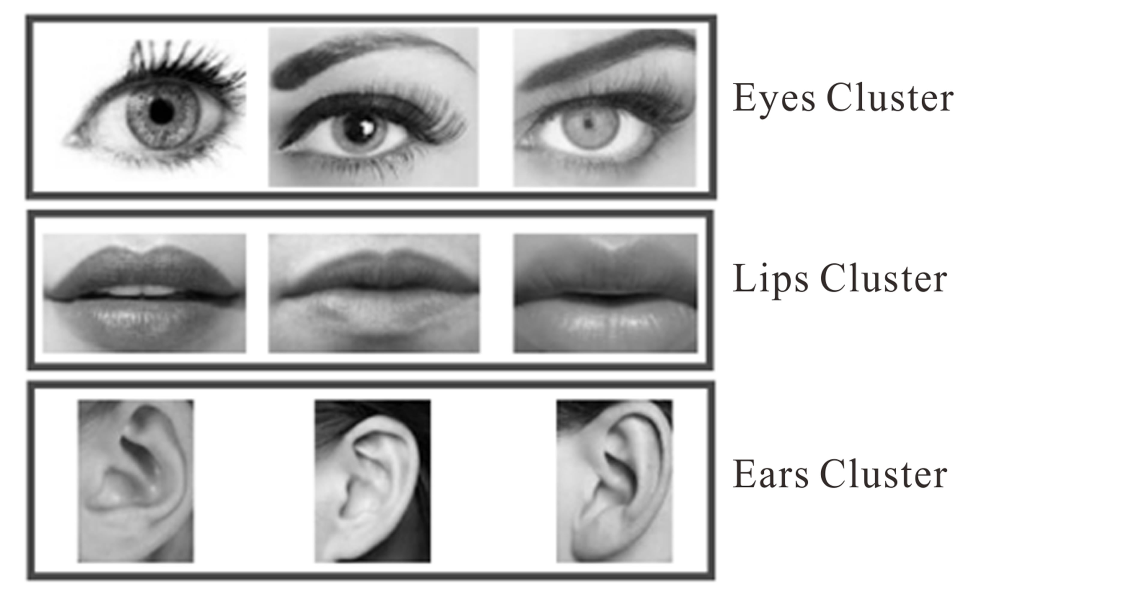
Figure 4. Clustering assembles all similar patterns, marked by 6 filters, in the related bins.
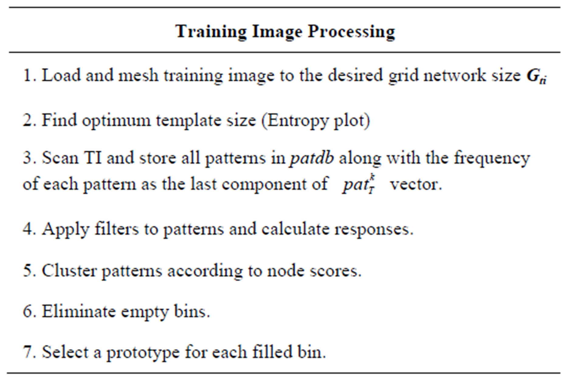
Table 2. Training image processing steps of the Modified FILTERSIM approach.
3. Facies Simulation
Simulation begins by defining a random path on realization nodes. Data event in the template is extracted in each node and its similarity to the existing patterns is then measured. Data event vector devT (u) is a set of previously informed nodes in unconditional simulation while hard data is also added to devT (u) in conditional simulation. Similarity between data event and extracted patterns in patdbT is measured by a distance (or difference) function .We used the following single point manhattan distance function:
 (4)
(4)
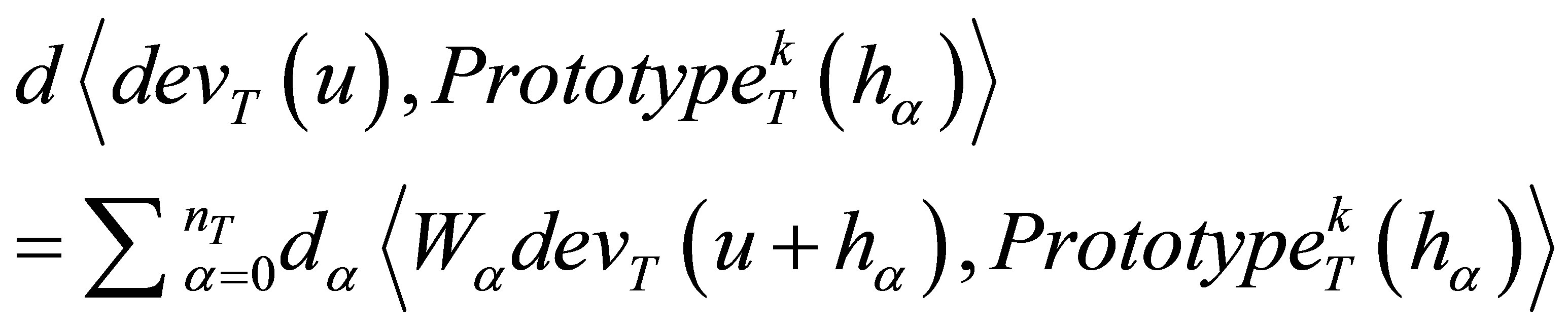
Having the random path defined, a search among the prototypes is done for each visited node to select the most similar prototype which shows minimum distance function  with data event as below:
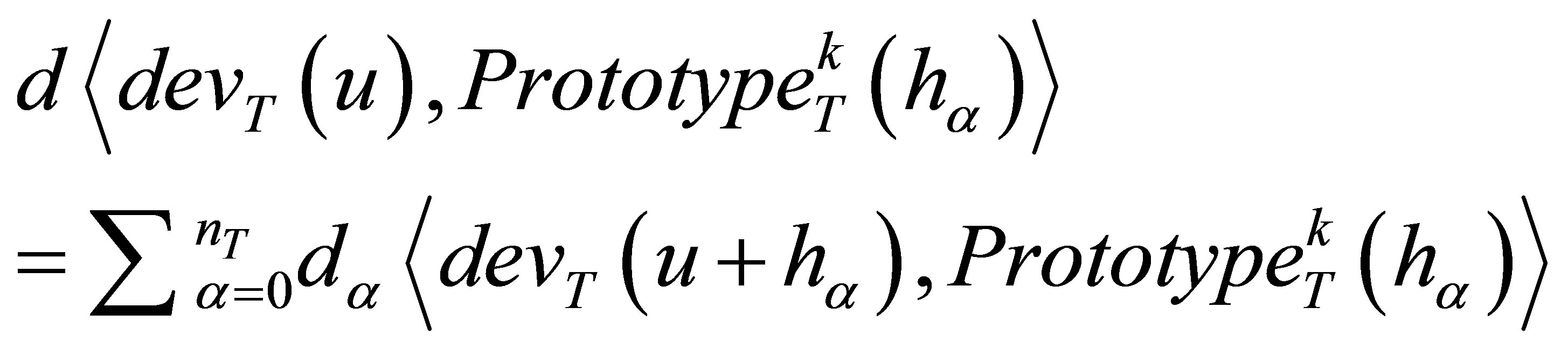 (5)
(5)
The bin of selected prototype contains the most similar patterns to the visited data event. FILTERSIM routine is to select a random pattern among these patterns and set it as realization node. This obviously is not the best procedure and may lose the feature connectivity as is a known drawback of this method. Here we modified the procedure and performed a second searching step to find the most similar pattern to data event in the selected bin (Figure 5). Pattern selection in candidate cluster is based on the following distance function:
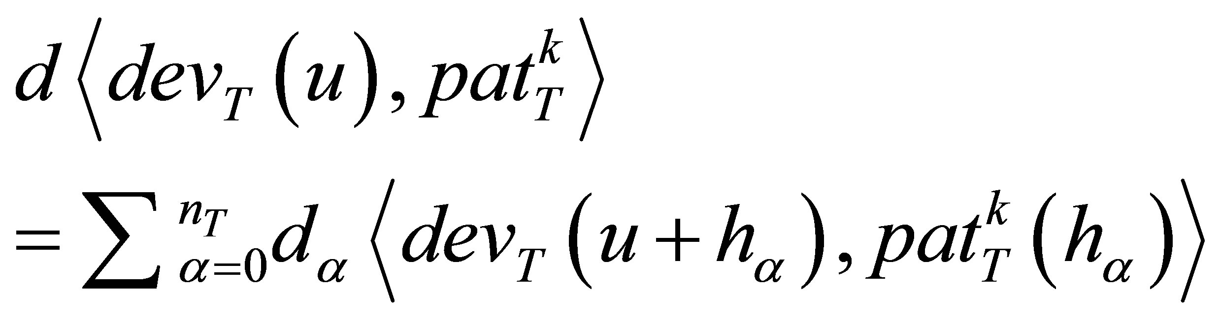 (6)
(6)
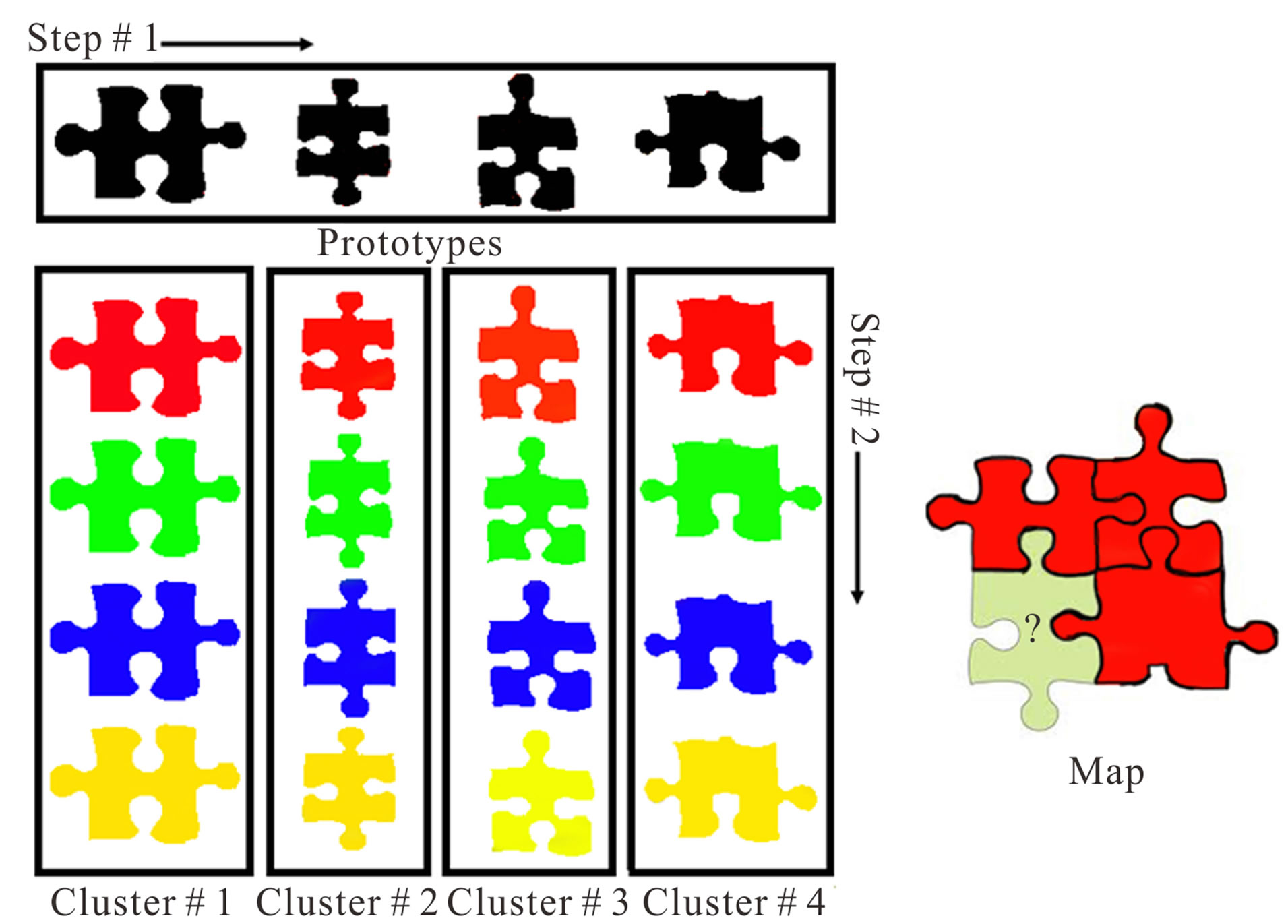
Figure 5. Schematic of searching between prototypes in Step # 1 and between selected cluster in Step # 2 (Step # 2 in FILTERSIM is random).
Only the pattern nodes with known values are considered in the above relation.
 (7)
(7)
The pattern with minimum distance function is then pasted entirely on realization nodes. If some patterns have the same distance to the data event vector, the one with the most frequency is selected. Random selection of patterns is only allowed when they all have the same frequency. This pattern selection strategy has improved the FILTERSIM performance and connectivity features of reconstructed realizations compare to the original method. This will be fully explored in the results section. Table 3 shows the stepwise procedure of Modified FILTERSIM approach described above.
The last but not the least point is the updatable region of pasted pattern on realization nodes which is used for the first time by Arpat in SIMAPT [1].The selected pattern after imposing on the visited node of realization is not entirely fixed and some outer parts of it can be replaced by future pasted patterns as shown in part 4 of Table 3. This provides the opportunity of superior realizations with closer features of connectivity to those of TI (Figure 6).
Conditional Simulation Algorithm
Data obtained from cores, wells and/or other exploration
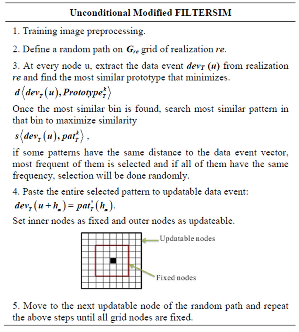
Table 3. Procedure steps of unconditional Modified FILTERSIM approach.
 (a) (b) (c)
Figure 6. Effect of updatable nodes on structures continuity: (a) training image, (b) realization with updatable region, (c) realization without updatable region.
sources are considered as hard data. These data are distinguished in TI and pattern data bank as hdevT (u). We are willing to reproduce hard data exactly in the realizations as they are occurred in the initial map. Unlike the other methods which are added additional searching steps, simulation algorithm we propose for realizations conditioned to hard data hdevT (u) is the same as unconditional simulation algorithm presented above, except to the distance function calculations for prototype selection. To do this, higher weights Wi, for the hard data are considered in distance function calculation while searching between prototypes.
 (8)
(8)
Hard data weights should be set according to their confidence level and accuracy. Satisfactory realizations were obtained with hard data weights four times bigger than the previously informed nodes as will be shown shortly in the result section. It is however necessary to set the same weights for hard and soft data events during the search among the patters within the selected bin to maintain features continuity in the reconstructed realization. If pattern data base is rich, hard data will be reproduced completely in visual appealing realization, otherwise training image is weak and algorithm cannot reproduce all the hard data in continuous structures. Simulation steps for conditional Modified FILTERSIM approach are summarized in Table 4.
Due to minimal changes in the main algorithm, no significant difference was observed in simulation time of conditional and unconditional cases.
4. Fracture Network Simulation
In fracture network images, fractures are thin and require very fine mesh to capture all spatial statistics. Having low CPU usage and continuous fractures, we apply a chamfer distance transform to the training image of fracture network. This transform can detect and extract main features of an image as shown in Figure 7. The image for this purpose should be a binary image.
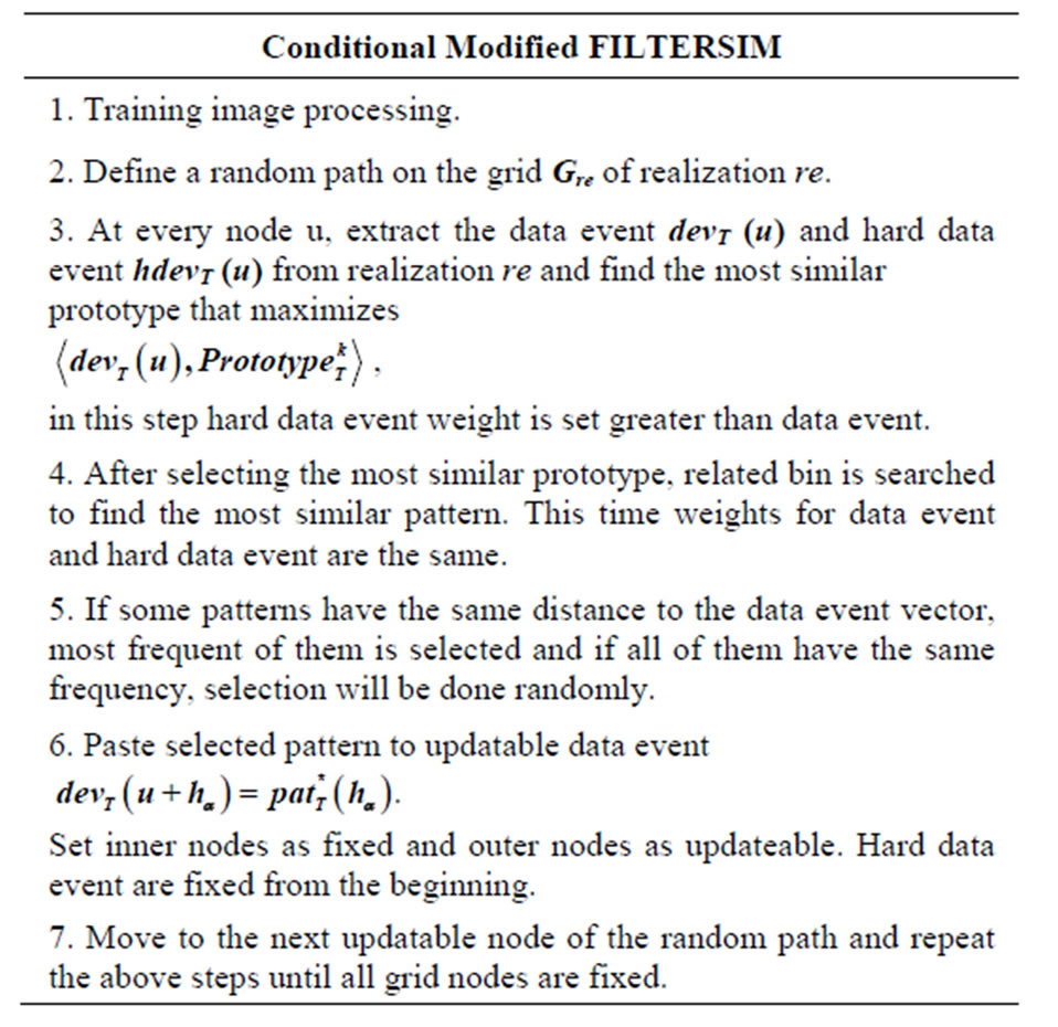
Table 4. Procedure steps of conditional Modified FILTERSIM approach.

Figure 7. Skeletonisation using chamfer distance transform.
Consider a binary fracture network image where fracture and matrix nodes are set to 1 and 0 respectively. Chamfer transform creates a continuous figure in which its node values reflect their distance to the target objects, i.e. fractures in our case. Node values decrease monotonically from 1 to 0 as their distance increase from fractures.
Chamfer transform for each node uα of the training image ti is:
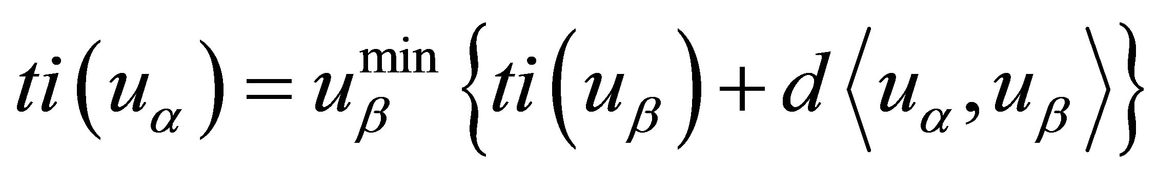 (9)
(9)
where uβ are the nodes within the template T with  Distance of uα to each neighbor node uβ is calculated and the value of ti (uβ) is added to this distance (which itself is a distance). Value of ti (uα) is set to the minimum of these distances. Figure 8 shows the chamfer transformed image of fracture network TI.
Modified FILTERSIM just described in Table 3 can now be applied to this transformed image.
Generated realizations are continuous values ranged from 0 to 1 similar to the transformed TI. This need to be back transformed to a binary image which simply possible by setting all the less than 1 node values to 0.
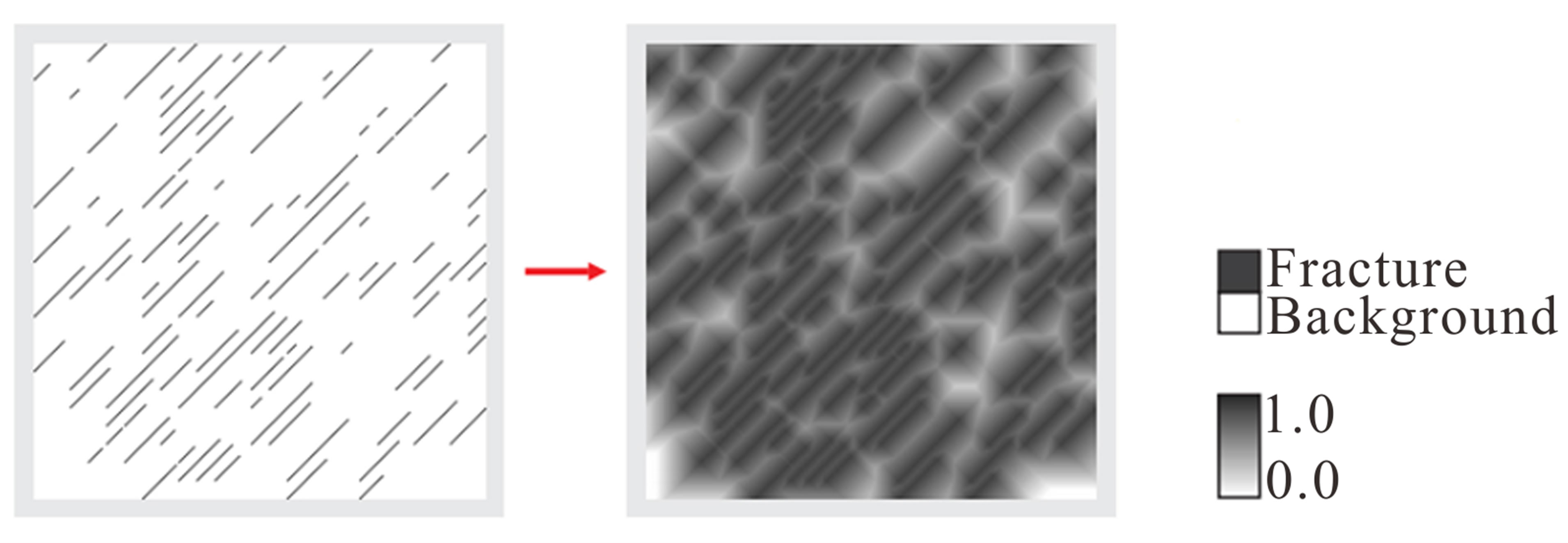
Figure 8. Application of chamfer proximity transform to the binary training image.
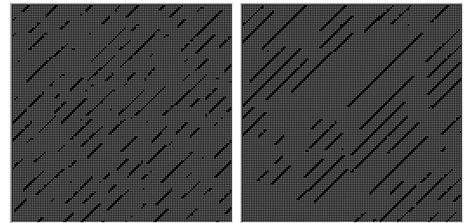
Figure 9 shows two generated realizations of fracture network TI of Figure 8. It is evident that chamfer transform as we applied considerably enhanced the realization and generated closer patters to the TI.
5. Multiple Grid Approach
Optimum template size in training image processing controlls realization richness in different scales. Multiple template sizes are however needed to capture geological structures with various heterogeneity patterns at several scales. To this end, we propose a multi grid approach in which the simulations are run for one size greater than, equal to, and smaller than the optimum template size. Simulation starts by the biggest template size. Node values from pervious steps are then considered as updatable soft data in the next simulations with smaller template sizes. Weights of these informed nodes considered as the half of those which informed in the current step for distance function calculations. This makes the small scale structures to better reconstruct on a large scale background as shown in Figure 10. Optimum template size of 13 is obtained for this TI. Realization with multiple grid approach used template sizes of 13, 11 and 9 after each other to better capture smaller scale heterogeneities as is evident in this figure.
6. Results and Discussion
Modifications are made to the original FILTERSIM algorithm in several ways of optimizing template size, considering pattern frequency component in database and pattern distance function ranking in candidate bin instead of random selection. Performance of this modified algorithm is investigated by applying the method on 2D training images with grid size of 128 × 128. Both unconditional and conditional situations are studied. Figure 11 compares reconstructed realizations of a binary TI at with unconditional algorithms of FILTERSIM, SIMPAT and Modified FILTERSIM. Better visual continuity of the Modified FILTERSIM result is clear. Algorithm Performance was also investigated by applying the method on continuous 2D training image (Figure 12).
Conditioning to hard data just marginally increases computations due to the simple and fast proposed meth-
 (a) (b)
Figure 9. Generated realizations (a) without and (b) with chamfer transformation ((a) structures are piecemeal, (b) have continues fractures and better reproduces the training image patterns).

Figure 10. Single grid and multiple grid simulation results.
odology. This is not the case for other methods as illustrated in Figure 13 which compares CPU simulation times of SIMPAT, original and Modified FILTERSIM approaches. Although computationally more expensive than FILTERSIM, the Modified FILTERSIM method is still far faster than SIMPAT and is superior in performance compare to the both methods.
Modified FILTERSIM performance for conditional reconstruction of TI is illustrated in Figure 14. Chanelly TI similar to that of Figure 11 is considered with 3 different hard data distributions. Several conditional realizations are generated for each hard data distribution. Averaging the results to E-type maps shows that all hard data are exactly reproduced in all realization as they are fixed in E-type maps of Figure 14.
It is worth to mention that parallel generation of several realizations is possible in our proposed algorithm. Our developed computer program can start several realizations simultaneously based on available computation cores and hardware characteristics. This considerable accelerate the simulations and makes the risk analysis and uncertainty management an easy task.
7. Summary
We proposed a MPS algorithm to simulate 2D binary and continuous stationary structures. Optimum template size for each training image is elaborated. This, along with a pattern frequency component in database and additional
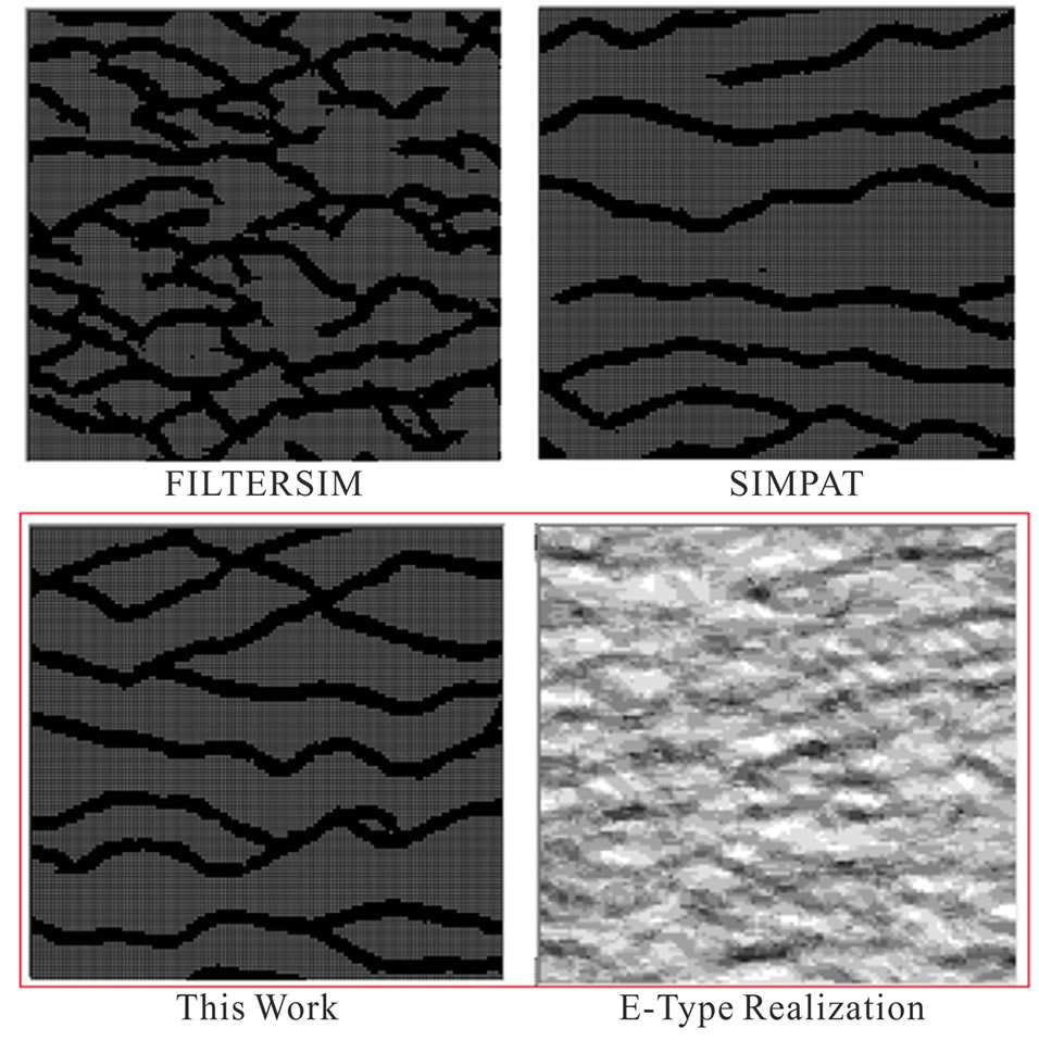
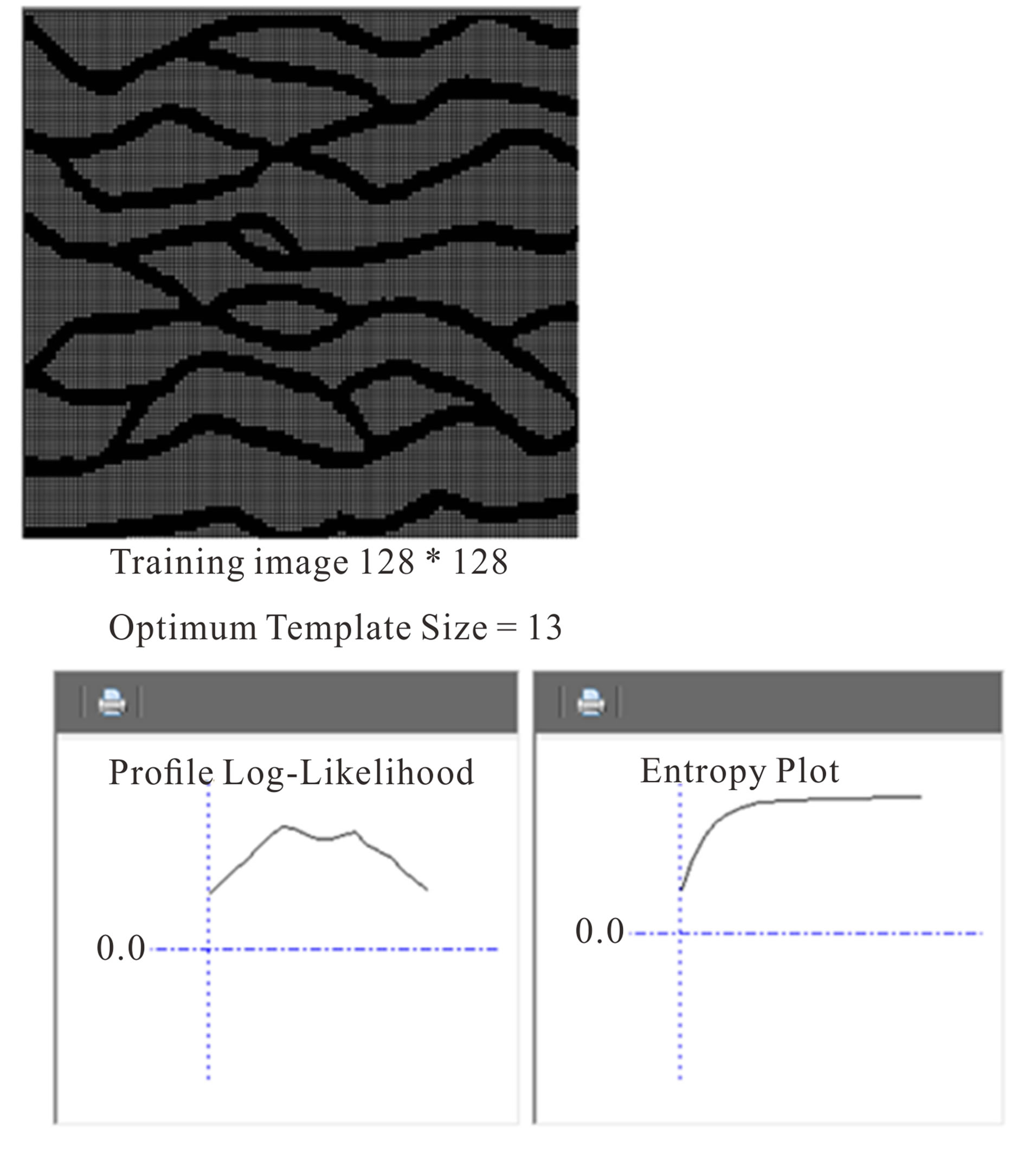
Figure 11. Simulation results by applying SIMPAT, FILTERSIM and this work method.
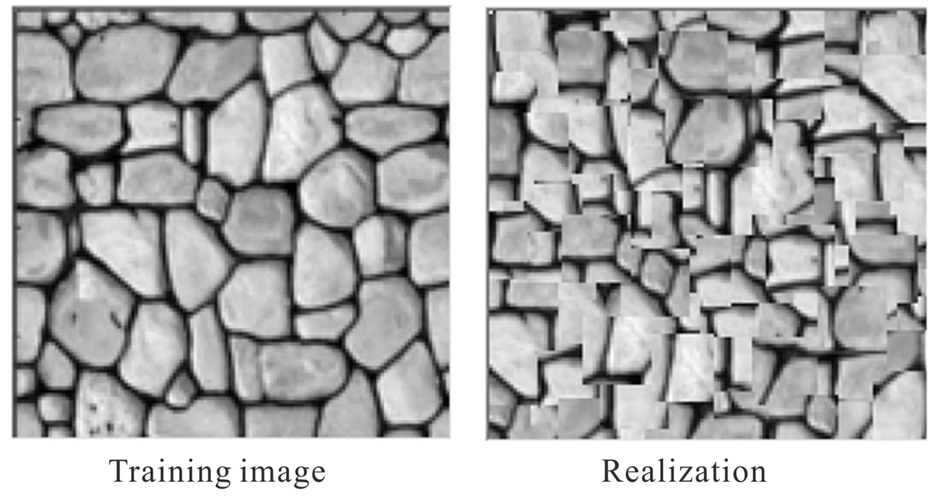
Figure 12. 2D continuous training image and simulation result (Optimum Template Size is 15).
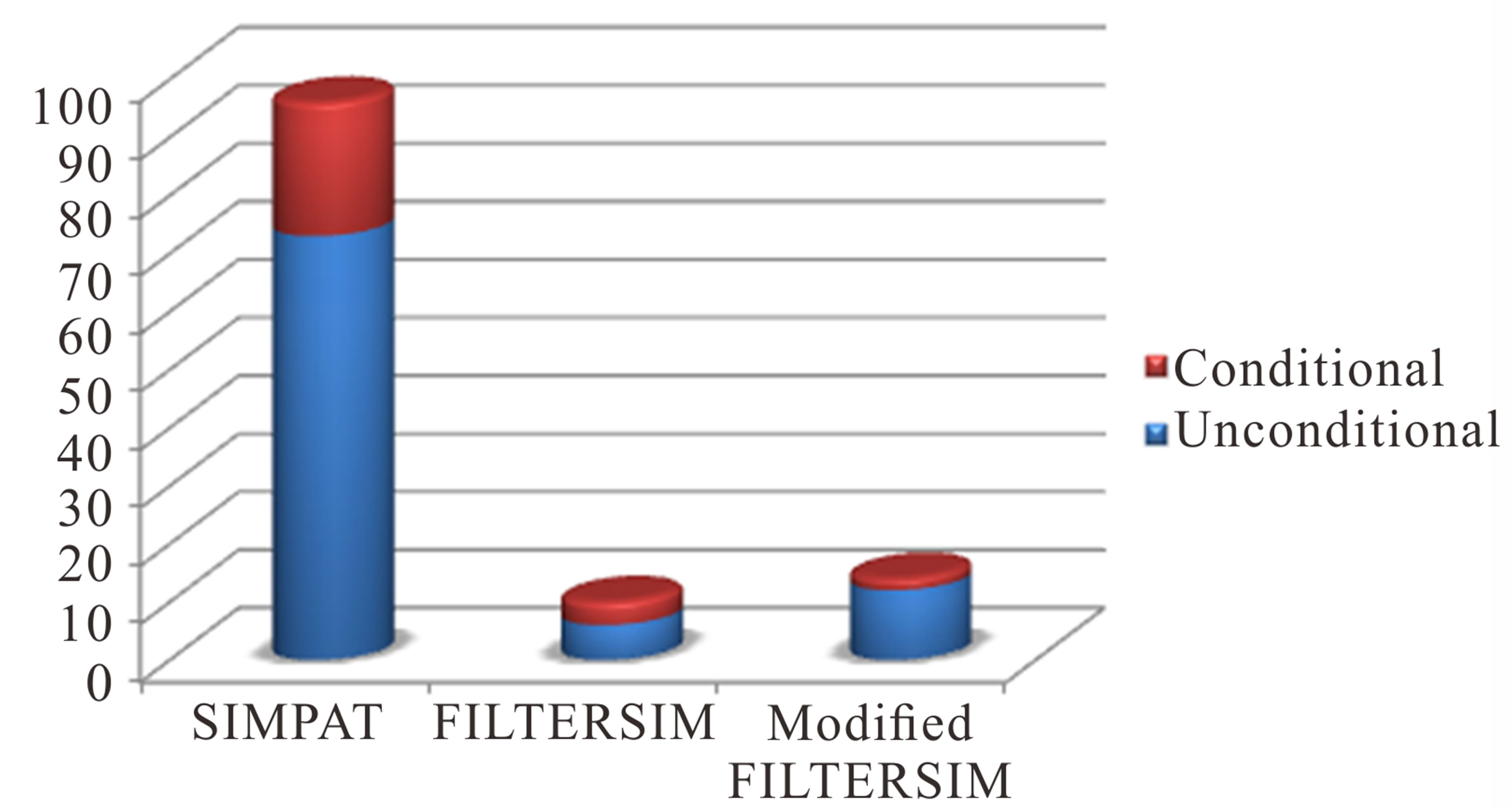
Figure 13. CPU Time Qualitative Comparison of SIMPAT, FILTERSIM and Modified FILTERSIM methods (Minimum increase in CPU time due to adding conditionality feature occurs in Modified FILTERSIM).
search among stored patterns in the selected bin, is shown to improve the FILTERSIM performance considerably. Shannon entropy concept was used to infer optimum template size that can capture local structures in each template. Frequency component increases the chance of more repeated patterns to be selected; prototypes and patterns are chosen based on their minimum Manhattan distance function with data events within the realization under construction. Several examples showed that our proposed algorithm can produce more visual-appealing
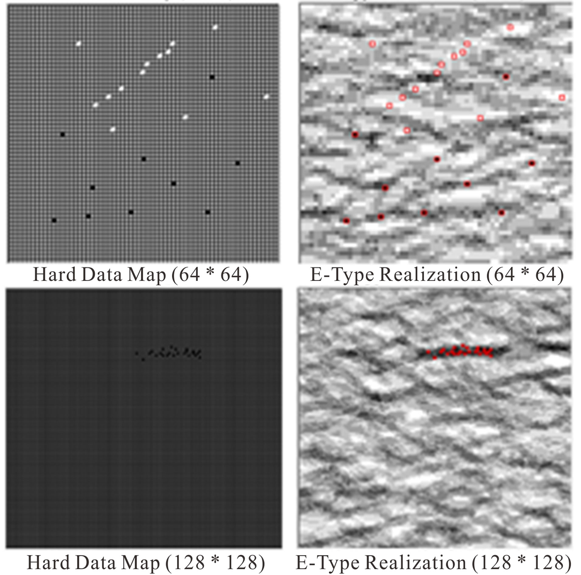
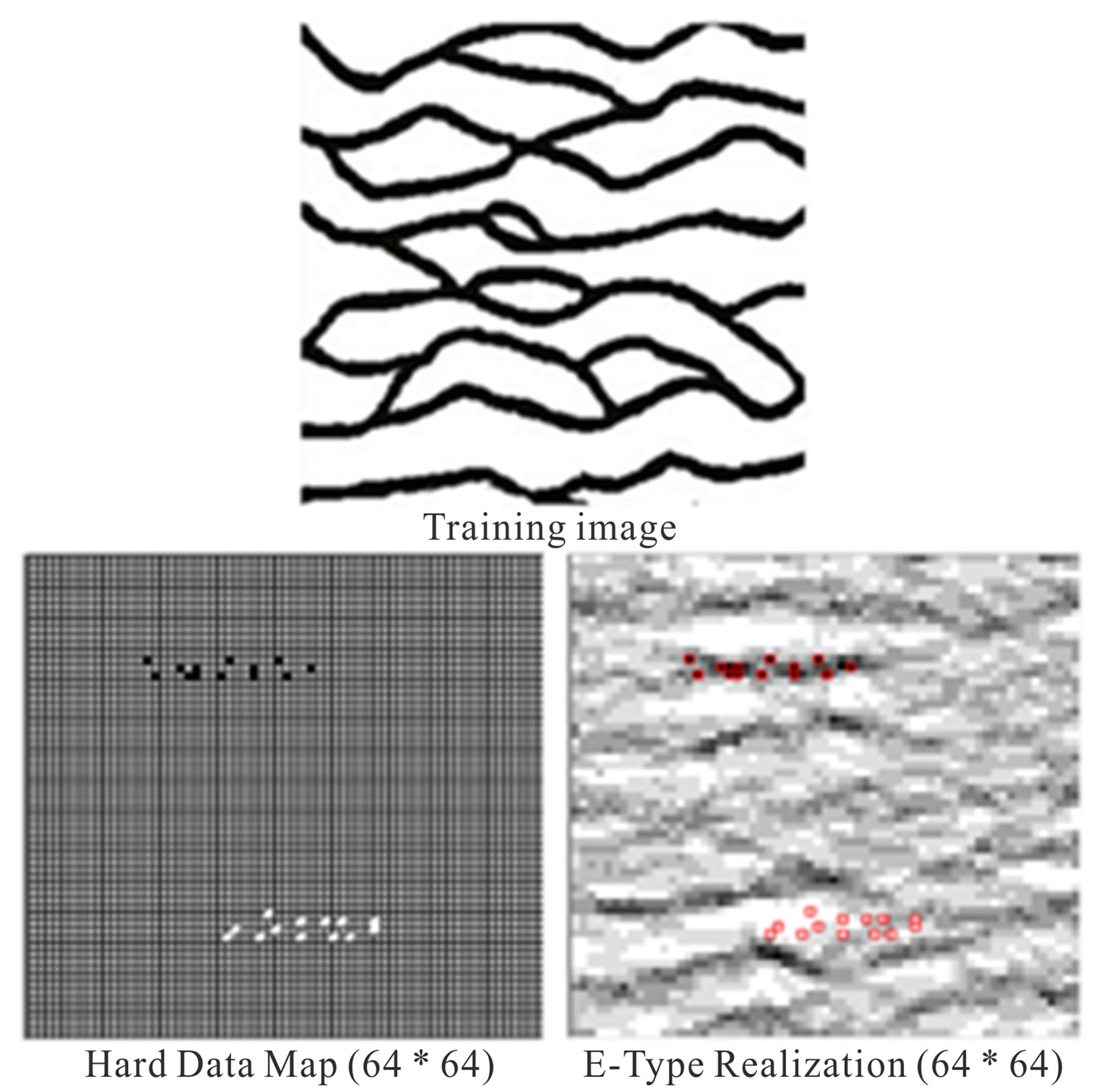
Figure 14. E-Type Realization obtained from 12 realizations by conditional Modified FILTERSIM.
images compared to both FILTERSIM and SIMPAT algorithms. These improvements add marginal computation cost to FILTERSIM and yet still much faster than SIM-PAT.
Chamfer transformation of TI for fractured rocks and simulation with multiple template sizes for complex structures with several heterogeneity scales make the performance of our Modified FILTERSIM algorithm even better.
Our algorithm, SIMPAT and original FILTERSIM have been implemented in C#. We have made our code stand alone and provided a user interface to upload TIs and to display simulation results. In the future, we plan to extend Modified FILTERSIM algorithm to non-stationary and 3D pore space structures. The later will be based on 2D real thin section images.
REFERENCES
- G. Arpat and J. Caers, “A Multiple-Scale, Pattern-Based Approach to Sequential Simulation,” 7th International Geostatistics Congress. GEOSTAT 2004 Proceedings, Banff, October 2004.
- S. Strebelle, “Conditional Simulation of Complex Geological Structures Using Multiple-Point Statistics,” Mathematical Geology, Vol. 34, No. 1, 2002, pp. 1-21. http://dx.doi.org/10.1023/A:1014009426274
- A. G. Journel and T. Zhang, “The Necessity of a Multiple-Point Prior Model,” Mathematical Geology, Vol. 38 No. 5, 2006, pp. 591-610.
- J. Ortiz, “Characterization of High Order Correlation for Enhanced Indicator Simulation,” Ph.D. thesis, University of Alberta, Edmonton, 2003.
- J. Boisvert, M. J. Pyrcz and C. V. Deutsch, “MultiplePoint Statistics for Training Image Selection,” Natural Resources Research, Vol. 16, No. 4. 2007.
- K. G. Boogaart, “Some Theory for Multiple Point Statistics: Fitting, Checking and Optimally Exploiting the Training Image,” International Association for Mathematical Geology 11th International Congress, 2006.
- F. Guardiano and M. Srivastava, “Multivariate Geostatistics: Beyond Bivariate Moments,” In: A. Soares, Ed., GeostatisticsTroia, Kluwer Academic Publications, Dordrecht, 1993, pp. 133-144.
- S. Strebelle, “Sequential Simulation Drawing Structures from Training Images,” Ph.D. Thesis, Stanford University, 2000.
- J. Straubhaar, P. Renard, G. Mariethoz, R. Froidevaux, and O. Besson, “An Improved Parallel Multiple-Point Algorithm Using a List Approach,” Mathematical Geosciences, Vol. 43, No. 3, 2011, pp. 305-328.
- J. Caers, “GEOSTATISTICS: From Pattern Recognition to Pattern Reproduction,” Developments in Petroleum Science, Vol. 51, 2003, pp. 97-115. http://dx.doi.org/10.1016/S0376-7361(03)80010-9
- X. Y. Liu, C. Y. Zhang, Q. S. Liu and J. Birkholzer, “Multiple-Point Statistical Prediction on Fracture Networks at Yucca Mountain,” 2004.
- M. J. Ronayne, S. M. Gorelick and J. Caers, “Identifying Discrete Geologic Structures That Produce Anomalous HyDraulic Response: An Inverse Modeling Approach,” Water Resources Research, Vol. 44, No. 8, 2008. http://dx.doi.org/10.1029/2007WR006635
- M. Stien, P. Abrahamsen, R. Hauge and O. Kolbjørnsen, “Modification of the Snesim Algorithm,” EAGE, Petroleum Geostatistics, 2007.
- M. Huysmans and D. Alain, “Application of Multiplepoint Geostatistics on Modelling Groundwater Flow and Transport in a Cross-Bedded Aquifer,” Hydrogeology Journal, Vol. 17, No. 8, 2009, pp. 1901-1911.
- H. Okabe and J. Blunt, “Pore Space Reconstruction Using Multiple-Point Statistics,” Journal of Petroleum Science and Engineering, Vol. 46, No. 1-2, 2005, pp. 121-137. http://dx.doi.org/10.1016/j.petrol.2004.08.002
- T. Zhang, P. Switzer and A. Journel, “Filter-Based Classification of Training Image Patterns for Spatial Simulation,” Mathematical Geology, Vol. 38, No. 1, 2006, pp. 63-80. http://dx.doi.org/10.1007/s11004-005-9004-x
- M. Honarkhah and J. Caers, “Stochastic Simulation of Patterns Using Distance-Based Pattern Modeling,” Mathematical Geosciences, Vol. 42, No. 5, 2010, pp. 487- 517. http://dx.doi.org/10.1007/s11004-010-9276-7
- M. Honarkhah and J. Caers, “Classifying Existing and Generating New Training Image Patterns in Kernel Space,” 21st SCRF Aliate Meeting, Stanford University, 2008.
- S. Chatterjee, R. Dimitrakopoulos and H. Mustapha, “Dimensional Reduction of Pattern-Based Simulation Using Wavelet Analysis,” Mathematical Geosciences Work to Be Submitted, 2011.
- P. Mohammadmoradi and M. Rasaei, “Modification of the FILTERSIM Algorithm for Unconditional Simulation of Complex Spatial Geological Structures,” Journal of Geomaterials, Vol. 2 No. 3, 2012, pp. 49-56.
- C. E. Shannon, “A Mathematical Theory of Communication,” Bell System Technical Journal, Vol. 27, 1948. pp. 379-423,623-656.