American Journal of Computational Mathematics
Vol.2 No.3(2012), Article ID:23187,4 pages DOI:10.4236/ajcm.2012.23027
Two Initial Value Problems Approach for Solving Singular Perturbations Problems
1Department of Mathematics, Bahir dar University, Bahir dar, Ethiopia
2National Institute of Technology, Warangal, India
Email: *awoke248@yahoo.com
Received May 18, 2012; revised June 23, 2012; accepted July 8, 2012
Keywords: Singular Perturbation; Initial Value Problems; Asymptotic Power Series Expansions
ABSTRACT
In this paper, we presented an initial value approach for solving singularly perturbed two point boundary value problems with the boundary layer at one end (left or right). By employing asymptotic power series expansion, the given singularly perturbed two-point boundary value problem is replaced by two first order initial value problems. To demonstrate the applicability of the present method three linear and two nonlinear problems with left end boundary layer are considered. It is observed that the present method approximates the exact solution very well.
1. Introduction
The theory of singular perturbations has been with us, in one form or another, for a little over a century (although the term “singular perturbation” dates from the 1940s). The subject, and the techniques associated with it, has evolved over this period as a response to the need to find approximate solutions (in an analytical form) to complex problems. Typically, such problems are expressed in terms of differential equations which contain at least one small parameter, and they can arise in many fields: fluid mechanics, particle physics and combustion processes, to name but three. The essential hallmark of a singular perturbation problem is that a simple and straightforward approximation (based on the smallness of the parameter) does not give an accurate solution throughout the domain of that solution. Perforce, this leads to different approximations being valid in different parts of the domain (usually requiring a “scaling” of the variables with respect to the parameter). This in turn has led to the important concepts of breakdown, matching, and so on.
Singularly perturbed second order two-point boundary value problems have been received a significant attention in past and recent years. These problems arise very frequently in fluid mechanics and other branches of Applied Mathematics. These problems depend on a small positive parameter in such a way that the solution varies rapidly in some parts and varies slowly in some other parts. So, typically there are thin layers where the solutions can jump abruptly, while away the layers the solution behaves regularly and vary slowly. Thus more efficient, simpler computational techniques are required to solve singular perturbation problems. Awoke A, Y. N. Reddy [1,2] presented the method of Asymptotic Inner Boundary Condition and a terminal boundary condition for Singularly Perturbed Two-Point Boundary value Problems. The papers by Kadalbajoo and Reddy [3], and Kadalbajoo and Patidar [4] give an erudite outline of the singular perturbation problems. The approach were characterized by using a terminal point, the original second order problem is divided in to two problems namely inner region and outer region problems. For more discussions, one can refer: Bender and Orsazag [5], Kevorkian and Cole [6], Nayfeh [7,8], O’Mally [9] and Van Dyke [10].
In this paper, a couple of initial-value problems for solving singularly perturbed two-point boundary value problems with the boundary layer at one end (left or right) point is presented. By employing asymptotic power series expansion, the given singularly perturbed two-point boundary value problem is replaced by two first order initial value problems. To demonstrate the applicability of the present method three linear and two nonlinear problems with left end boundary layer are considered. Table of absolute maximum error is presented and it is observed that the present method approximates the exact solution very well for step size (h) significantly larger than the perturbation parameter (ε).
2. A Pair of Initial Value Problems
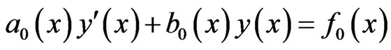
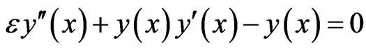
Consider a linear singularly perturbed two-point boundary value problem of the form:
 (1)
(1)
with
 (2a)
(2a)
and
 (2b)
(2b)
where e is a small positive parameter ( ) and a, b are known constants. We assume that
 ,
,  and
and  are sufficiently continuously differentiable functions in [0, 1] and that the problem has a unique solution
 . Further more, we assume that
  exhibits a boundary layer at left end of the interval [0, 1].
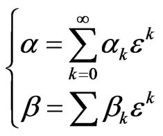
We assume that ,
,  and
and  have asymptotic power series expansions of the form:
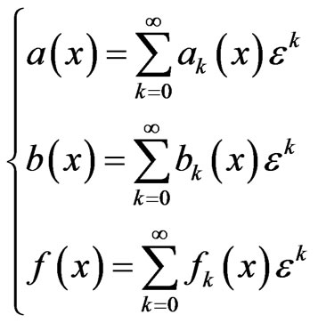 (3a)
(3a)
and
 (3b)
(3b)
for suitable smooth functions ,
,  and
and  and suitable constants
  and
and . The reduced problem by taking
  in (10.1) is:
 with
with 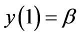 (4)
(4)
From the theory of singular perturbation, it is possible to find a two-variable expansion for y in the form:
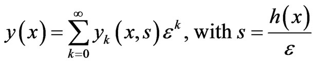 (5)
(5)
where the function h is at our disposal subject to the conditions that it be strictly monotonic and vanish at , i.e.
 ,
, . A possible choice for h includes
 and
and . For details one can refer Smith ([11] pages 287-289). Substituting the expansions (5) and (3a) in to Equation (1), the equation for the coefficients
  will take the form:
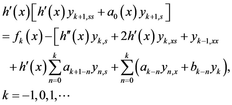 (6)
(6)
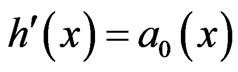
where the right side of (6) is understood to be zero when the value for k = −1. For this case let us choose the function , which satisfies the above conditions. And then we have
 (7)
(7)
By substituting (7) in to (6), we get
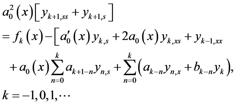 (8)
(8)
where again the right side of (8) is put equal to zero in the case of k = −1.
We can solve Equation (8) recursively with respect to s, for each fixed x. For k = −1, we get
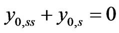 (9)
(9)
The solution of (9) for suitable quantities U0, V0 which still depend on x is given by:
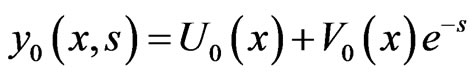 (10)
(10)
We now insert (10) back to the right side of (8) with k = 0 and we get the differential equation for y1:
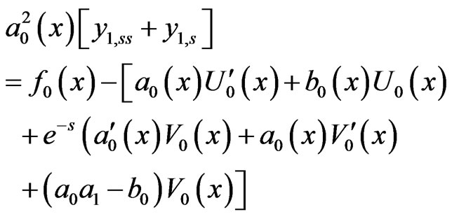 (11)
(11)
If we take the right side of (11) to be zero, we get
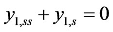 (12)
(12)
Its solution takes the form
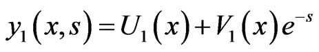 (13)
(13)
for suitable function  and
and  dependent only on x.
This procedure can be continued recursively, and we get in general,
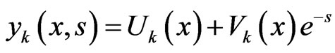 (14)
(14)
for suitable function  and
and  dependent only on x.
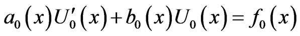
Here to find an approximate solution for y of Equations (1) and (2), we are taking the right side of (11) equal to zero and we get two initial value problems of the form:
 (15a)
(15a)
and
 (15b)
(15b)
In order to set up the boundary condition to solve Equations (15), we insert (10) in to (3b) and we get
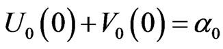 (16a)
(16a)
and
 (16b)
(16b)
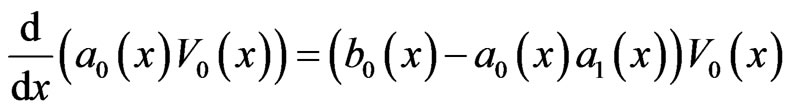
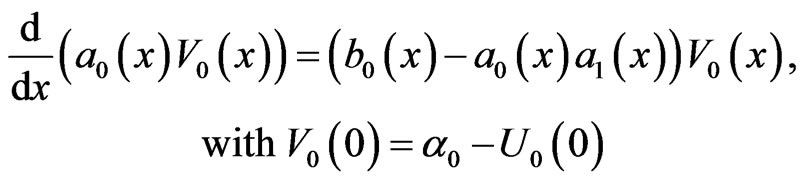
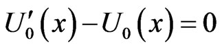
Now we solve the following pair of initial value problems:
 , with
 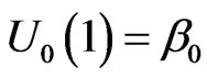 (17a)
(17a)
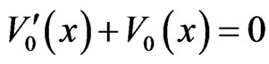
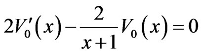
and
 (17b)
(17b)
Finally the approximate solution for (1) and (2) is determined by using (17) and (10).
3. Numerical Examples
Three linear singular perturbation problems with left-end boundary layer were considered to demonstrate the applicability of the present method (Table 1).
Example 3.1: Consider the following homogeneous singular perturbation problem from Bender and Orszag ([5], page 480; problem 9.17 with a = 0)
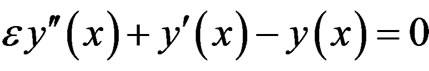 ;
; , with
  and
and .
.
The two initial value problems are:
 , with
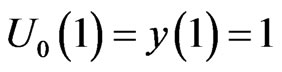
 , with
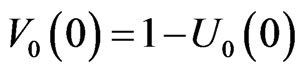
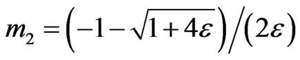
The exact solution is given by:
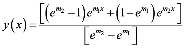
where 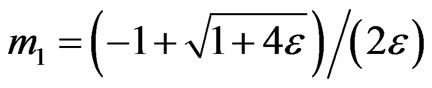 and
and
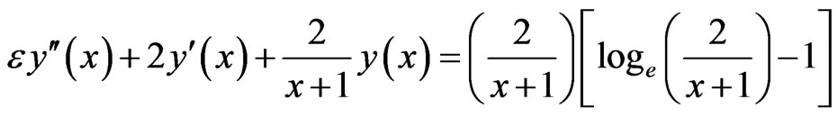
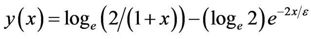
Example 3.2: Now consider the following non-homogeneous singular perturbation problem from fluid dynamics for fluid of small viscosity, Reinhardt ([12], example 2)
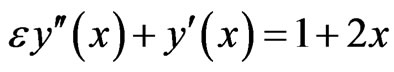 ;
; , with
 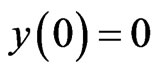 and
and .
.
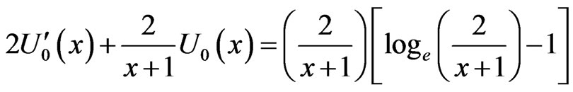
The two initial value problems are:
 , with
 , with
Example 3.3: Finally we consider the following variable coefficient singular perturbation problem from Kevorkian and Cole [6], page 33; equations (2.3.26) and (2.3.27) with a = −1/2]
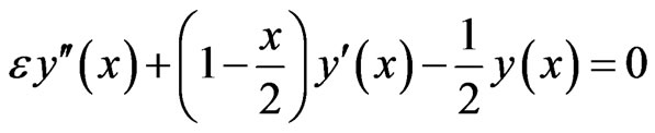 ;
; , with
  and
and .
.
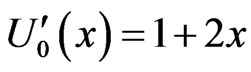
The two initial value problems are:
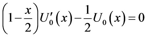 , with
 , with
We have chosen to use uniformly valid approximation (which is obtained by the method given by Nayfeh ([7], page 148; equation (4.2.32)) as our “exact” solution:
4. Nonlinear Examples
The method of Quasilinearization is used to solve the nonlinear singular perturbation problems (Table 1).
Example 4.1: Consider the following singular perturbation problem from Bender and Orszag ([5], page 463; equation (9.7.1))
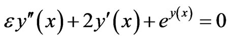 ;
; , with
  and
and .
.
The linear problem concerned to this example is
The two initial value problems are:
 , with
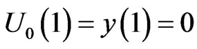
 , with
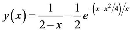
We have chosen to use Bender and Orszag’s uniformly valid approximation ([3], page 463; equation (9.7.6)) for comparison,
For this example, we have boundary layer of thickness  at x = 0 (cf. Bender and Orszag [5]).
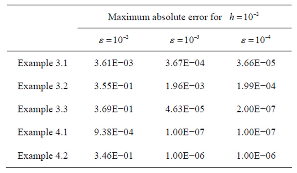
Table 1. Maximum absolute error.
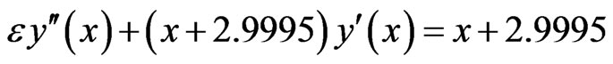
Example 4.2: Consider the following singular perturbation problem from Kevorkian and Cole ([6], page 56; equation (2.5.1))
 ;
; , with
  and
and 
The linear problem concerned to this example is
The two initial value problems are:
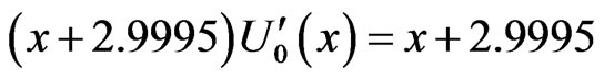 , with
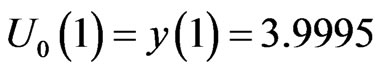
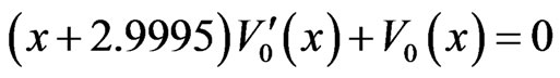 , with
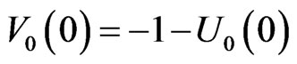
We have chosen to use the Kevorkian and Cole’s uniformly valid approximation [6], pages 57 and 58; equations (2.5.5), (2.5.11) and (2.5.14) for comparison,
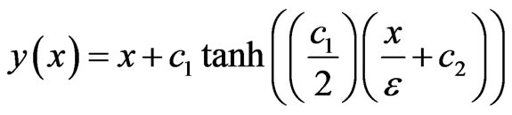
where c1 = 2.9995 and 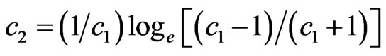
For this example also we have a boundary layer of width  at x = 0 (cf. Kevorkian and Cole [6], pages 56-66).
5. Discussion and Conclusion
Converting the second order boundary value problem in to the corresponding first order initial value problems is always preferable as the numerical solution of a boundary value problem will be more difficult than getting the numerical solution of initial value problems. The solution of the given singularly perturbed two-point boundary value problem is computed numerically by solving pair of initial value problems. The applicability of the present method is tested by considering three linear and two nonlinear problems with left end boundary layer by taking different values of e. To solve the pair of initial value problems we used the classical fourth order Runge-Kutta method. Table of absolute maximum error is presented, which shows that the present method approximates the exact solution very well for step size (h) significantly larger than the perturbation parameter (e).
REFERENCES
- A. Awoke and Y. N. Reddy, “The Method of Asymptotic Inner Boundary Condition for Singular Perturbation Problems,” Journal of Applied Mathematics & Informatics, Vol. 29, No. 3-4, 2011, pp. 937-948.
- A. Awoke and Y. N. Reddy, “Terminal Boundary Condition for Singularly Perturbed Two-Point Boundary Value Problems,” Neural, Parallel and Scientific Computations, Vol. 16, No. 3, 2008, pp. 435-448.
- M. K. Kadalabajoo and Y. N. Reddy, “Asymptotic and Numerical Analysis of Singular Perturbation Problems: A Survey,” Applied Mathematics and Computation, Vol. 30, No. 3, 1989, pp. 223-259. doi:10.1016/0096-3003(89)90054-4
- M. K. Kadalbajoo and K. C. Patidar, “A Survey of Numerical Techniques for Solving Singularly Perturbed Ordinary Differential Equations,” Applied Mathematics and Computation, Vol. 130, No. 2-3, 2002, pp. 457-510. doi:10.1016/S0096-3003(01)00112-6
- C. M. Bender and S. A. Orsazag, “Advanced Mathematical Methods for Scientists and Engineers,” Springer, New York, 1999.
- J. Kevorkian and J. D. Cole, “Perturbation Methods in Applied Mathematics,” 2nd Edition, Springer-Verlag, New York, 1981.
- A. H. Nayfeh, “Introduction to Perturbation Techniques,” Wiley-VCH, New York, 1993.
- A. H. Nayfeh, “Perturbation Methods,” John Wiley & Sons, Inc., New York, 1979.
- R. E. O’Malley, “Introduction to Singular Perturbations,” Academic Press, New York, 1974.
- M. D. Van Dyk, “Perturbation Methods in Fluid Mechanics,” Parabolic Pr, New York, 1975.
- D. R. Smith, “Singular Perturbation Theory: An Introduction with Applications,” Cambridge University Press, Cambridge, 1985.
- H.-J. Reinhardt, “Singular Perturbations of Difference Methods for Linear Ordinary Differential Equations,” Applicable Analysis, Vol. 10, No. 1, 1980, pp. 53-70. doi:10.1080/00036818008839286
NOTES
*Corresponding author.