ABSTRACT

This paper introduces an interval valued linear fractional programming problem (IVLFP). An IVLFP is a linear fractional programming problem with interval coefficients in the objective function. It is proved that we can convert an IVLFP to an optimization problem with interval valued objective function which its bounds are linear fractional functions. Also there is a discussion for the solutions of this kind of optimization problem.

1. Introduction

While modeling practical problems in real world, it is observed that some parameters of the problem may not be known certainly. Specially for an optimization problem it is possible that the parameters of the model be inexact. For example in a linear programming problem we may have inexact right hand side values or the coefficients in objective function may be fuzzy (e.g. [1]).

There are several approaches to model uncertainty in optimization problems such as stochastic optimization and fuzzy optimization. Here we consider an optimization problem with interval valued objective function. Stancu, Minasian and Tigan ([2,3]), investigated this kind of optimization problem. Hsien-Chung Wu ([4,5]) proved and derived the Karush-Kuhn-Tucker (KKT) optimality conditions for an optimization problem with interval valued objective function.

A fractional programming problem is the optimizing one or several ratios of functions (e.g. [6]). Such these models arise naturally in decision making when several rates need to be optimized simultaneously such as production planning, financial and corporate planning, health care and hospital planning. Several methods were suggested for solving this problem such as the variable transformation method [7] and the updated objective function method [8]. Several new methods are proposed ( e.g. [9-11]). The first monograph [12] in fractional programming published by the first author in 1978 extensively covers applications, theoretical results and algorithms for single-ratio fractional programs (see [13,14]).

Here first we introduce a linear fractional programming problem with interval valued parameters. Then we try to convert it to an optimization problem with interval valued objective function.

In Section 2 we state some required preliminaries from interval arithmetic. In Section 3 the interval valued linear fractional programming problem is introduced. In Section 4 we solved numerical examples. Finally Section 5 contains some conclusions.

2. Preliminaries

We denote by the set of all closed and bounded intervals in. Suppose, then we write and also. We have the following operations on (note that throughout this paper our intervals considered to be bounded and closed):

(i)

(ii) ;

(iii)

where is a real number and so we have

Definition 2.1. If and are bounded, real intervals, we define the multiplication of and as follows:

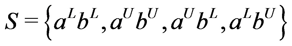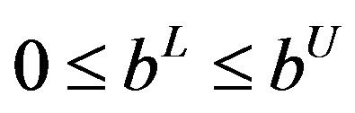where. For example if and are positive intervals (i.e. and) then we have:

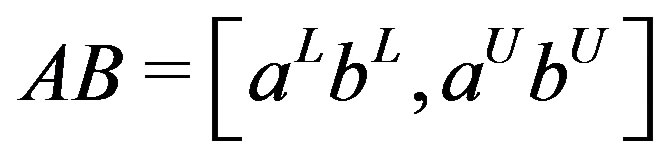(1)

and if 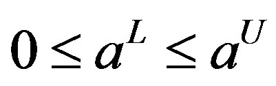and then we have:

(2)

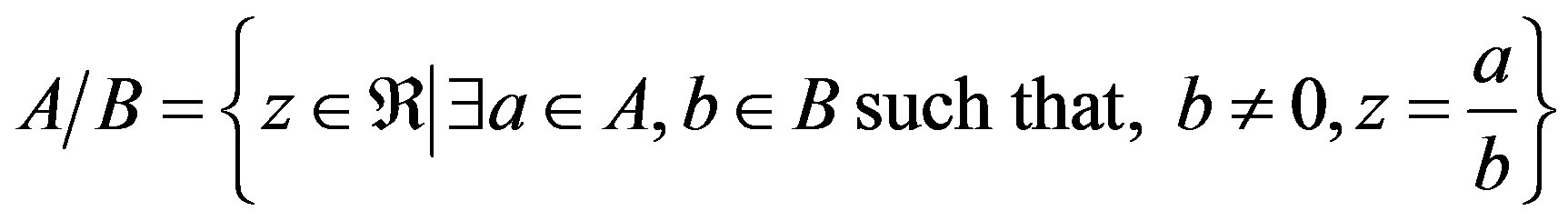
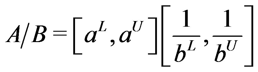
There are several approaches to define interval division. Following Ratz (see [15]) we define the quotient of two intervals as follows:

Definition 2.2. Let and be two real intervals, then we define:

We observe that the quotient of two intervals is a set which may not itself be an interval. For example,. Given definition 2.2, The Ratz formula [15] is given by the following Theorem:

Theorem 2.1. ([15]) Let and

be two nonempty bounded real intervals.

Then if we have:

(3)

Theorem 2.2. (see [16]) If and are nonempty, bounded, real intervals, then so are, and. In addition, if does not contain zero, then is also a nonempty, bounded, real interval as well.

Definition 2.3. A function is called an interval valued function (because for each is a closed interval in). Similar to interval notation, we denote the interval valued function with where for every

are real valued functions and

Proposition 2.1. Let be an interval valued function defined on. Then is continuous at if and only if and are continuous at c.

Now, here we introduce weakly differentiability.

Definition 2.4. Let be an open set in. An interval valued function with

is called weak differentiable at if the real valued functions and are differentiable (usual differentiability) at.

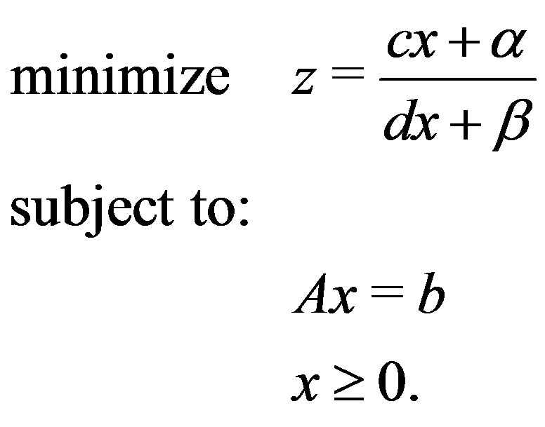
Definition 2.5. We define a linear fractional function as follows:

(4)

where and are real scalars.

Remark 2.1. Note that every real number can be considered as an interval.

Definition 2.6. To interpret the meaning of optimization of interval valued functions, we introduce a partial ordering over I. Let, be two closed, bounded, real intervals, then we say that, if and only if and. Also we write, if and only if and. In the other words, we say if and only if:

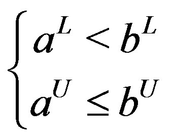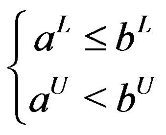or or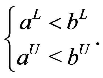

3. Interval-Valued Linear Fractional Programming (IVLFP)

Consider the following linear fractional programming problem:

(5)

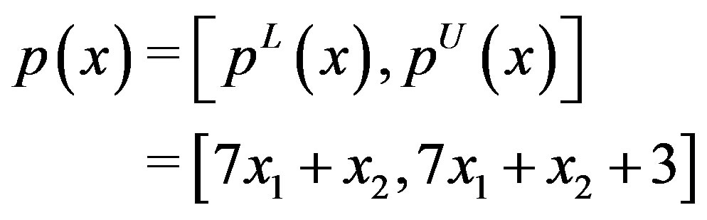
First consider the linear fractional programming problem (5). Suppose that

where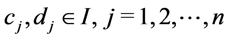, we denote and the lower bounds of the intervals and respectively (i.e. and also

where and are real scalars for) and, similarly we can define and. Also,. So we can rewrite (5) as follows:

(6)

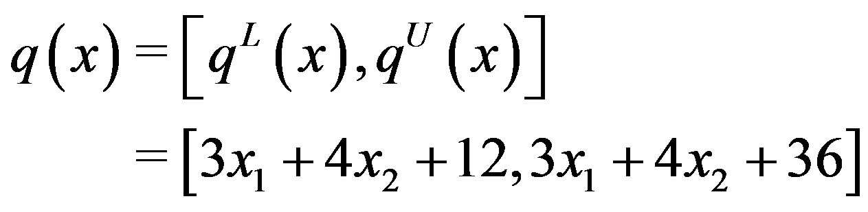
where and are interval-valued linear functions as

and. So for example we have: 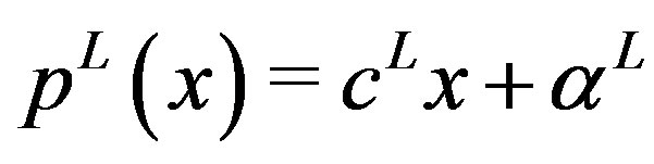and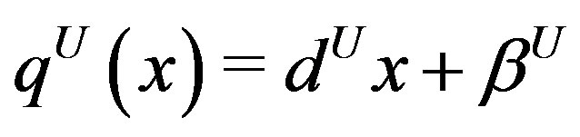. Finally from (6) we have:

(7)

To introduce an interval-valued linear fractional programming problem, we can consider another kind of possible linear fractional programming problems as follows:

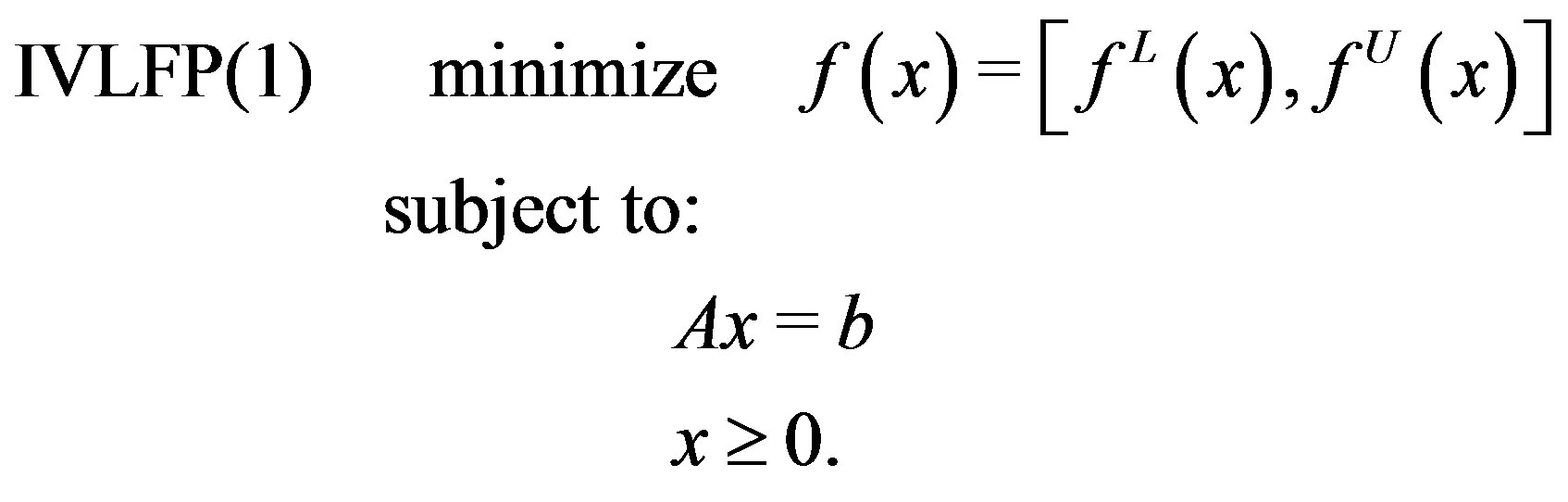(8)

where and are linear fractional functions (as in definition 2.5). Also we may have interval-valued linear fractional programming in the form (7):

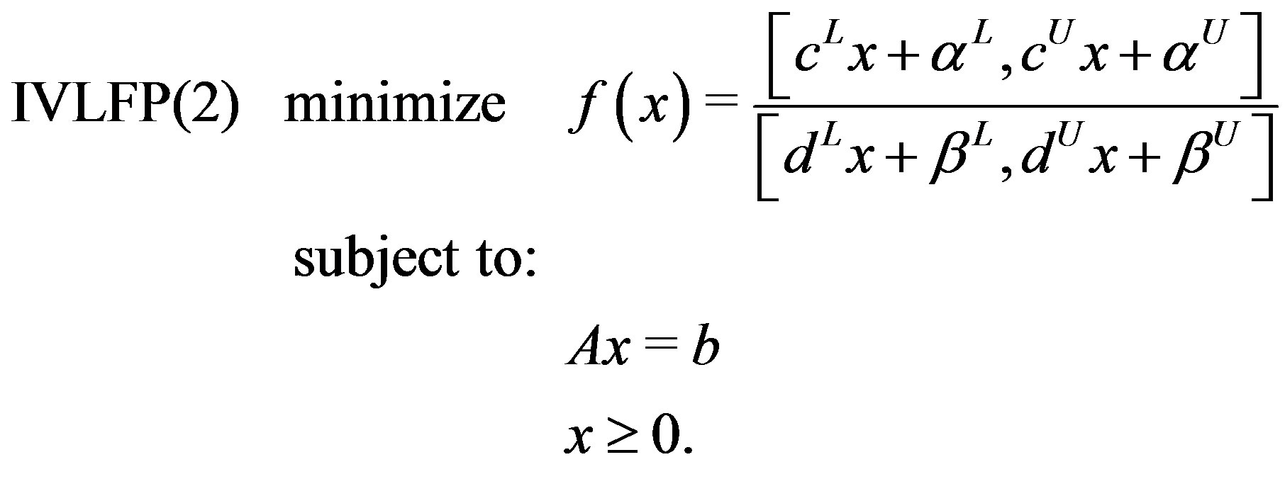(9)

Theorem 3.1. Any IVLFP in the form IVLFP(2) (see Equation (9)) under some assumptions can be converted to an IVLFP in the form IVLFP(1) (see Equation (8)).

Proof. The objective function in (9) is a quotient of two interval valued functions (and). To convert (9) to the form (8), we suppose that for each feasible point, so we should have:

(10)

or

(11)

for each feasible point. Using theorem 2.1, because the denominator doesn’t contain zero we can rewrite the objective function in (9) as:

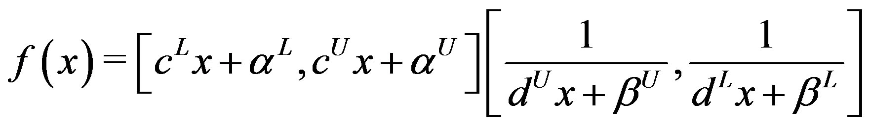(12)

Now we can consider two possible states:

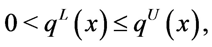
Case (1). When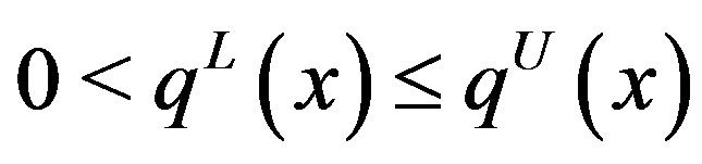, we have two possibilities:

(i) When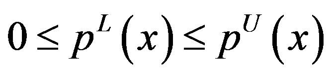, using Definition 2.1, we have:

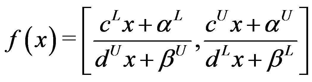(13)

(ii) When, by Definition 2.1, we have:

(14)

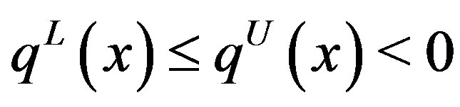
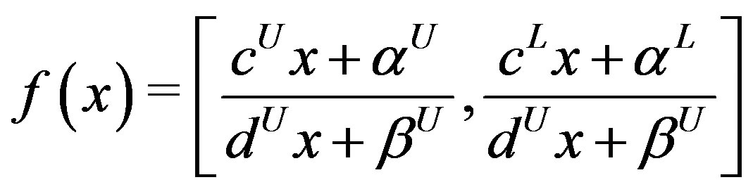
Case (2). When, we have two possibilities:

(i) When, by Definition 2.1, we have:

(15)

(ii) When, by Definition 2.1, we have:

(16)

(Note that the subcase 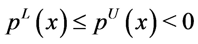easily can be derived from above cases, because in this state, implies that). Now according to theorem 2.2, and considering above cases, the objective function in (7) can be rewritten as follows:

(17)

where the objective function is an interval valued function and and are linear fractional functions (according to the corresponding case (13) - (16)), and this completes the proof.

Now following Wu [5], we interpret the meaning of minimization in (17):

Definition 3.1. (see [5]) Let be a feasible solution of problem (17). We say that is a nondominated solution of problem (17), if there exist no feasible solution x such that. In this case we say that is the nondominated objective value of.

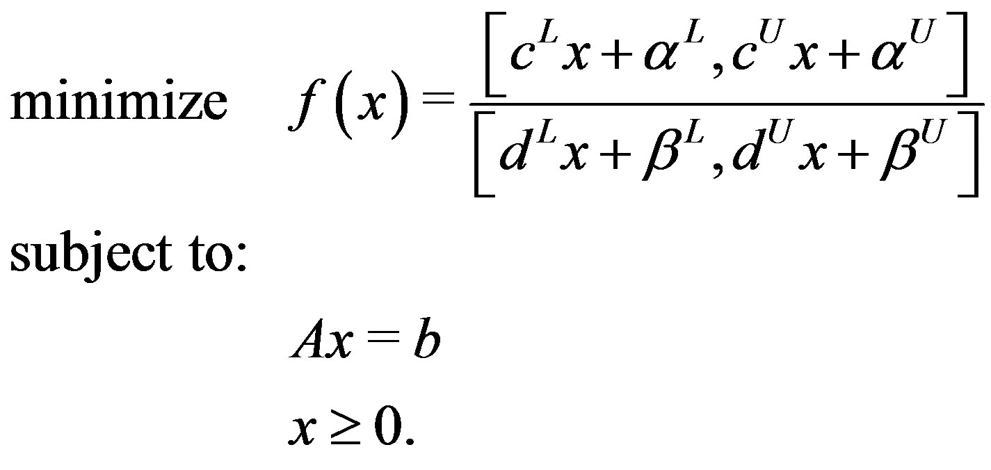
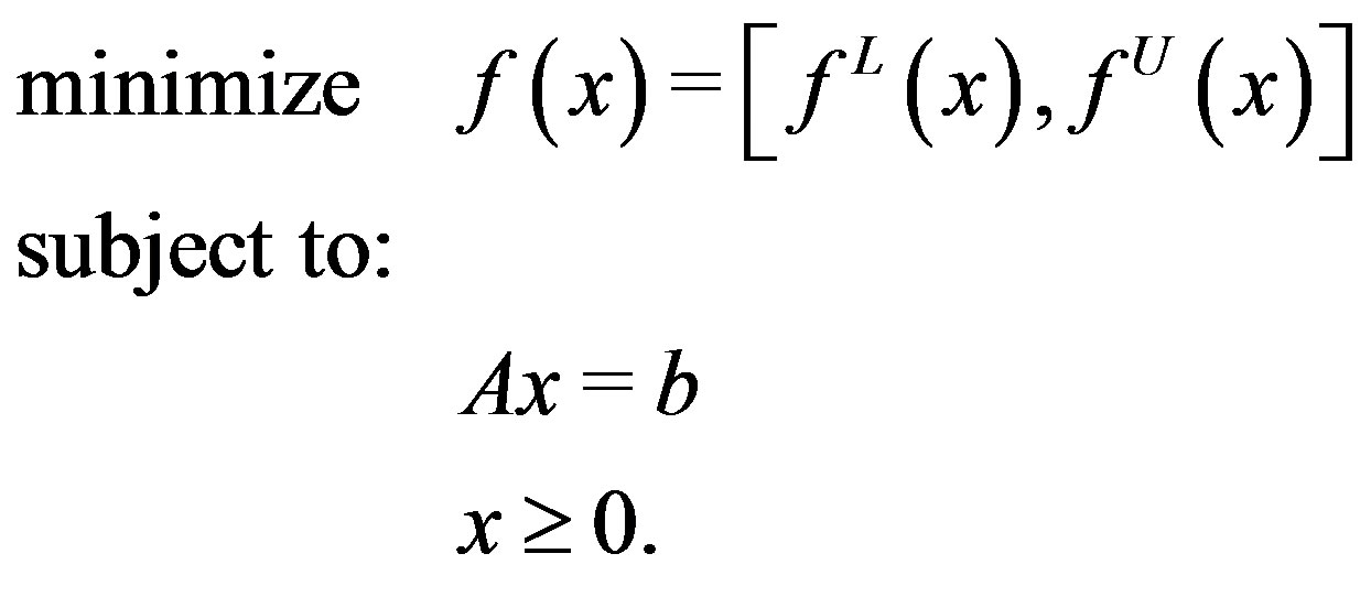
Now consider the following optimization problem (corresponding to problem (17)):

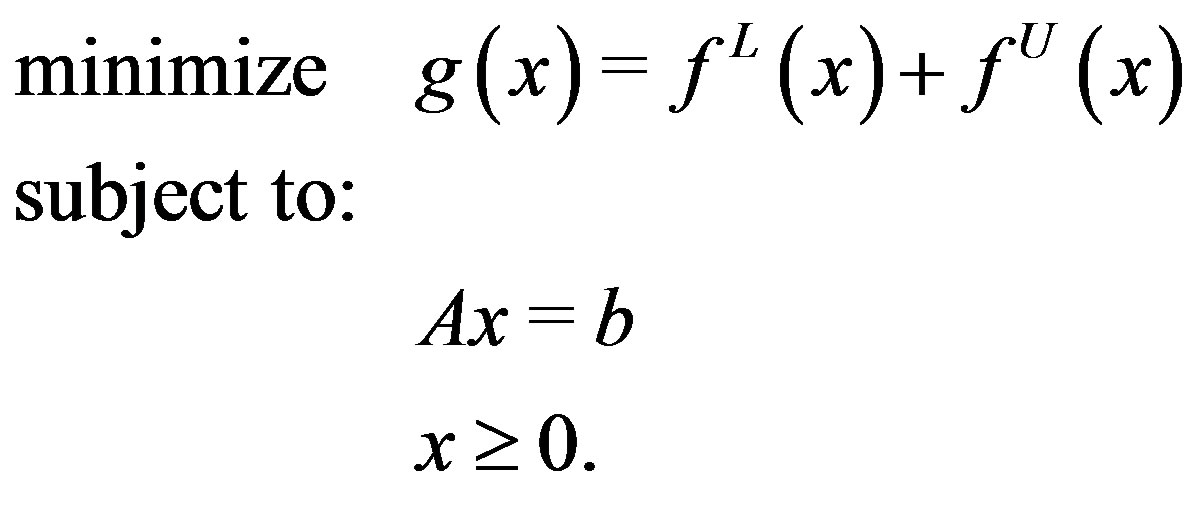(18)

To solve problem (17), we use the following theorem from [5].

Theorem 3.2. If is an optimal solution of problem (18), then is a nondominated solution of problem (17).

Proof. See [5].

4. Numerical Examples

This section contains three numerical examples which are solved by the new proposed approach. Example 4.3 introduces an application of IVLFP.

Example 4.1. Consider the following optimization problem:

(19)

We see that here

and

.

So because we have and also so we should apply case (1)(i). Finally we will have the following optimization problem:

(20)

Now to obtain a nondominated solution for (20), we use theorem 3.2. and solve the following optimization problem:

(21)

The optimal solution is 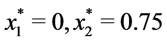with optimal value.

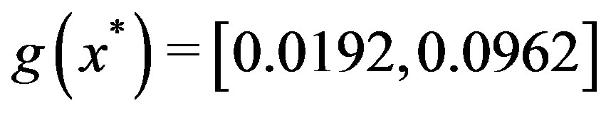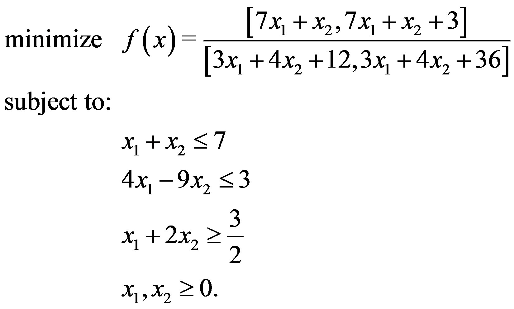
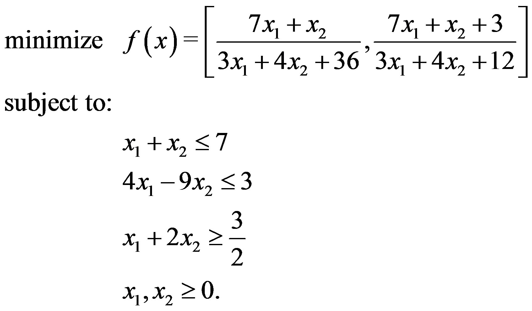
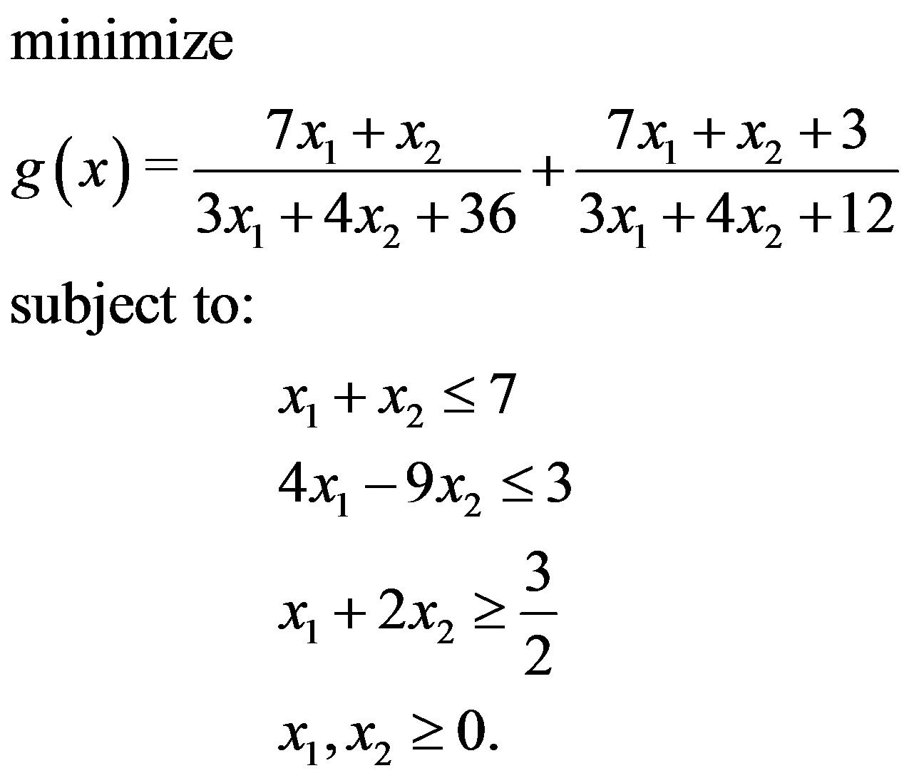
Example 4.2. Now consider the following optimization problem:

(22)

By Theorem 3.1, we can convert (22) to the following problem:

(23)

Now we can apply Theorem 3.2, and solve the optimization problem:

(24)

Finally a nondominated solution for (22) is

with

, which is the optimal solution of (24).

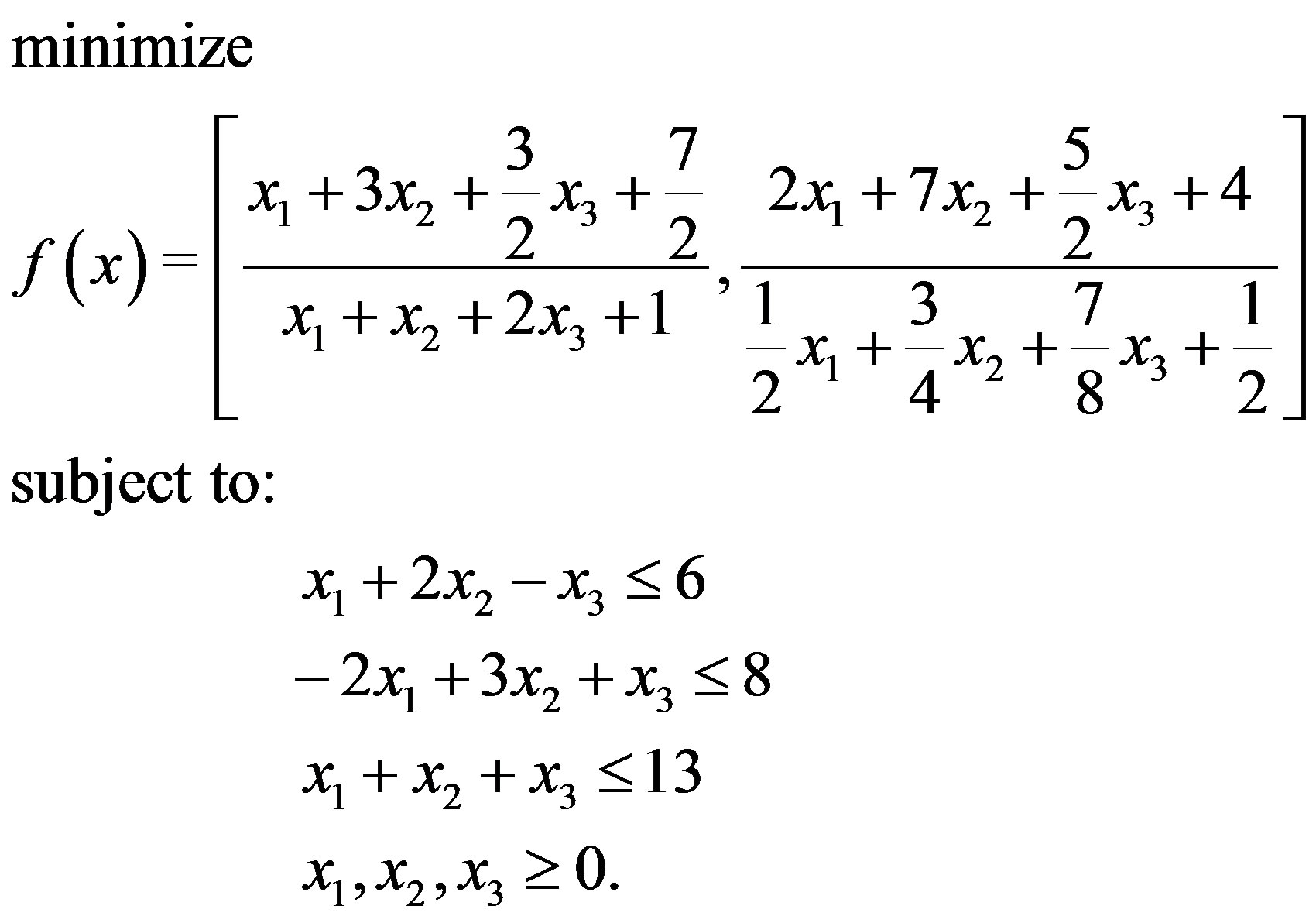
Example 4.3. Consider the following applied problem from [17]:

A company manufactures two kinds of products, with a uncertain profit of, dollar per unit respectively. .However the uncertain cost for each one unit of the above products is given by, dollar. It is assumed that a fixed cost of dollars is added to the cost function due to expected duration through the process of production and also a fixed amount of dollar is added to the profit function. If the objectives of this company is to maximize the profit in return to the total cost, provided that the company has a raw materials for manufacturing and suppose the material needed per pounds are 1, 3 and the supply for this raw material is restricted to 30 pounds, it is also assumed that twice of production of is more than the production of at most by 5 units. In this case if we consider and to be the amount of units of, to be produced then the above problem can be formulated as

(25)

The optimal solution is, with the objective value

5. Conclusion

In this paper, first we introduced two possible types (Equations (8), (9)) of linear fractional programming problems with interval valued objective functions. Then we proved that we can convert the problem of the form (9) to the form (8). By solving (8), we obtained a nondominated solution for original linear fractional programming problem with interval valued objective function. Work is in progress to apply and check the approach for solving nonlinear fractional programming problems as well as for quadratic fractional programming problems.

REFERENCES

- H. Ohta and T. Yamaguchi, “Linear Fractional Goal Programming in Consideration of Fuzzy Solution,” European Journal of Operational Research, Vol. 92, No. 1, 1996, pp. 157-165. doi:10.1016/0377-2217(95)00052-6
- I. M. Stancu-Minasian, “Stochastic Programming with Multiple Objective Functions,” D. Reidel Publishing Company, Dordrecht, 1984.
- I. M. Stancu-Minasian and St. Tigan, “Multiobjective Mathematical Programming with Inexact Data,” Kluwer Academic Publishers, Boston, 1990, pp. 395-418.
- H.-C. Wu, “The Karush-Kuhn-Tucker Optimality Conditions in an Optimization Problem with Interval-Valued Objective Function,” European Journal of Operational Research, Vol. 176, No. 1, 2007, pp. 46-59. doi:10.1016/j.ejor.2005.09.007
- H.-C. Wu, “On Interval-Valued Nonlinear Programming Problems,” Journal of Mathematical Analysis and Applications, Vol. 338, No. 1, 2008, pp. 299-316. doi:10.1016/j.jmaa.2007.05.023
- I. M. Stancu-Minasian, “Fractional Programming,” Kluwer Academic Publishers, Dordrecht, 1997.
- A. Charnes and W. W. Cooper, “Programs with Linear Fractional Functions,” Naval Research Logistics Quarterly, Vol. 9, No. 3-4, 1962, pp. 181-196. doi:10.1002/nav.3800090303
- G. R. Bitran and A. G. Novaes, “Linear Programming with a Fractional Function,” Operations Research, Vol. 21, No. 1, 1973, pp. 22-29. doi:10.1287/opre.21.1.22
- S. F. Tantawy, “A New Procedure for Solving Linear Fractional Programming Problems,” Mathematical and Computer Modelling, Vol. 48, No. 5-6, 2008, pp. 969-973. doi:10.1016/j.mcm.2007.12.007
- P. Pandey and A. P. Punnen, “A Simplex Algorithm for Piecewise-Linear Fractional Programming Problems,” European Journal of Operational Research, Vol. 178, No. 2, 2007, pp. 343-358. doi:10.1016/j.ejor.2006.02.021
- H. Jiao, Y. Guo and P. Shen, “Global Optimization of Generalized Linear Fractional Programming with Nonlinear Constraints,” Applied Mathematics and Computation, Vol. 183, No. 2, 2006, pp. 717-728. doi:10.1016/j.amc.2006.05.102
- S. Schaible, “Analyse und Anwendungen von Quotientenprogrammen, Ein Beitrag zur Planung mit Hilfe der Nichtlinearen Programmierung,” Mathematical Systems in Economics, Vol. 42, Hain-Verlag, Meisenheim, 1978.
- S. Schaible, “Fractional Programming: Applications and Algorithms,” European Journal of Operational Research, Vol. 7, No. 2, 1981, pp. 111-120. doi:10.1016/0377-2217(81)90272-1
- S. Schaible and T. Ibaraki, “Fractional Programming, Invited Review,” European Journal of Operational Research, Vol. 12, No. 4, 1983, pp. 325-338. doi:10.1016/0377-2217(83)90153-4
- D. Ratz, “On Extended Interval Arithmetic and Inclusion Isotonicity,” Institut fur Angewandte Mathematik, University Karlsruhe, 1996.
- T. Hickey, Q. Ju and M. H. Van Emden, “Interval Arithmetic: From Principles to Implementation,” Journal of the ACM, Vol. 48, 2001, pp. 1038-1068.
- S. F. Tantawy, “An Iterative Method for Solving Linear Fraction Programming (LFP) Problem with Sensitivity Analysis,” Mathematical and Computational Applications, Vol. 13, No. 3, 2008, pp. 147-151.