American Journal of Operations Research
Vol. 2 No. 3 (2012) , Article ID: 22415 , 9 pages DOI:10.4236/ajor.2012.23038
Almost Stochastic Dominance and Efficient Investment Sets
Jerusalem School of Business, The Hebrew University, Jerusalem, Israel
Email: mslm@huji.ac.il
Received July 8, 2012; revised August 10, 2012; accepted August 24, 2012
Keywords: Stochastic Dominance; Efficient Investment Set; Investment Choice
ABSTRACT
A major drawback of Mean-Variance and Stochastic Dominance investment criteria is that they may fail to determine dominance even in situations when all “reasonable” decision-makers would clearly prefer one alternative over another. Levy and Leshno [1] suggest Almost Stochastic Dominance (ASD) as a remedy. This paper develops algorithms for deriving the ASD efficient sets. Empirical application reveals that the improvement to the efficient sets implied by ASD is substantial (64% reduction for FSD). Direct expected utility maximization shows that investment portfolios excluded from the ASD efficient set would not have been chosen by any investors with reasonable preferences.
1. Introduction
The most popular tool for portfolio optimization and selection is the Mean-Variance (MV) analysis. The MV criterion conforms to Expected Utility (EU) maximization in the special case of normal return distributions1. Moreover, if rates of return are relatively small in absolute value, MV provides a good approximation for EU maximization, even when the return distributions are not normal (see Levy and Markowitz [5], and Markowitz [6]). In all other cases, the MV criterion may lead to choices contradicting EU maximization, and the selection criteria corresponding to EU maximization are the Stochastic Dominance (SD) criteria2.
The MV and SD efficient sets are important tools which allow the investor or investment company to narrow down the menu of relevant investments under consideration: inefficient investments should not be selected by any investor (in a given class of preferences), and therefore one can safely focus only on investments in the efficient set. Thus, it is not surprising that the MV and SD efficient investment sets have been the focus of many studies3. It is clear that the smaller the efficient set, the more helpful the investment criterion4.
While MV and SD are the most widely used investment criteria, they both suffer from the following drawback. Both the MV and SD criteria may fail to determine dominance even in situations where all “reasonable” investors would clearly prefer one investment to another. For instance, consider the following rather extreme example: suppose prospect G yields a return of 2% with a probability of  and a return of 3% with a probability of
 . Prospect F yields a return of 1% with a probability of
  and a return of 100% with a probability of
 . There is no MV or SD dominance of one prospect over the other in this case, i.e. both F and G are in the efficient MV and SD sets5. However, it is obvious that any “reasonable” investor would prefer investment F. Thus, a serious drawback of the standard investment criteria is that they do not exclude from the efficient set investments which “common sense” tells us that no real-world investor would ever select6.
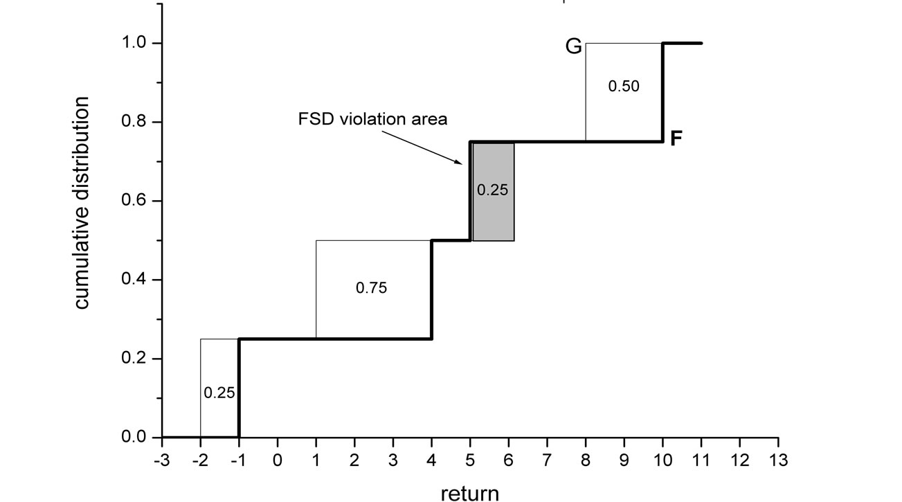
The Almost Stochastic Dominance (ASD) and Almost Mean-Variance (AMV) criteria, developed by Leshno and Levy [1], provide a solution to such paradoxical situations7. The idea at the heart of ASD can be graphically presented by Figure 1, which describes the cumulative return distributions of prospects F and G in the example above. The cumulative distribution of F is almost entirely below of the cumulative distribution of G. Thus, F “almost” dominates G by First-order Stochastic Dominance (FSD). However, there is a small “violation” region where F is above G, and therefore there is no FSD dominance of F. Another way to present the nondominance of F over G is to state that there are various “pathological” non-decreasing utility functions that yield higher expected utility under G. The idea of ASD is that if the area between the two cumulative distributions that causes the violation of FSD (area A1 in Figure 1) is very small relative to the total area enclosed between the two distributions (A1 + A2), then a dominance relationship holds for all “reasonable” investors. Thus, ASD describes dominance for the set of all “reasonable” preferences, excluding extreme preferences that are considered “pathological”. Although the ASD criterion is fairly recent, it has been already employed in several studies8.
This paper investigates two questions: 1) How significant is the reduction of the efficient sets obtained by employing ASD? And 2) What are the characteristics of the “pathological” preferences excluded? The paper is organized as follows. In the next section we review the Almost FSD (AFSD) and Almost SSD (ASSD) criteria. In Section 3 we develop algorithms for determining AFSD and ASSD dominance for empirical return distributions (with n return observations). In Section 4, we construct the AFSD and ASSD efficient sets for the 100 Fama-French portfolios, and we compare these sets with the standard FSD and SSD efficient sets. This section also investigates the degree to which preferences have to be “pathological” to be excluded from the ASD preference set. Section 5 concludes.
2. The Almost Stochastic Dominance Criteria
We discuss and employ two Almost SD criteria: AFSD (Almost First degree SD) and ASSD (Almost Second degree SD).
2.1. AFSD
Consider two alternative investments, F and G with cumulative distributions F(t) and G(t), respectively. Denote
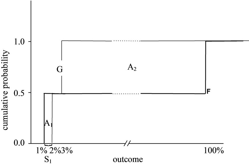
Figure 1. A graphic explanation of ASD. Investment G yields a return of 2% with a probability of  and a return of 3% with a probability of
 . Investment F yields a return of 1% with a probability of
  and a return of 100% with a probability of
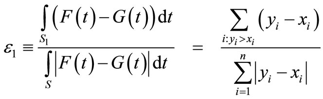
 . While it is clear that any “reasonable” investor would prefer F, F does not dominate G by FSD, because the small area A1 prevents FSD dominance. ε1 is defined as the ratio between the violation area and the total area enclosed between the two distributions:
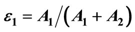 . F ε1-AFSD dominates G.
the range of possible outcomes (for both prospects) by S. F dominates G by FSD if and only if F(t) ≤ G(t) for all  (with at least one strict inequality). Almost FSD dominance of F over G means that F(t) ≤ G(t) for most of the range S, except for a relatively small segment that “violates” the dominance. Define the range over which FSD is violated by S1:
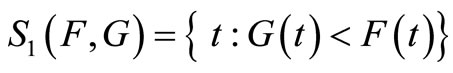 . (1)
. (1)
Denote the ratio between the area of FSD violation and the total area between the cumulative distributions by ε1:
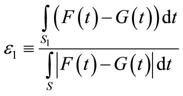 (2)
(2)
For ε1 < 0.5 F is said to “ε1-Almost FSD dominate” G. The smaller ε1, the stronger this dominance. Leshno and Levy [1] prove that if F ε1-Almost FSD dominates G then EFu ≥ EGu for all preferences , where
  is the set of all “well-behaved” or “reasonable” non-decreasing utility functions, given by:
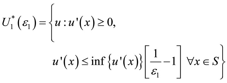 (3)
(3)
Note that for a given range S, the smaller the relative area violation, ε1, the larger the set of preferences . When ε1 = 0, i.e. there is no violation area at all,
  coincides with the usual set of all non-decreasing utility functions, U1, and AFSD reduces to the standard FSD criterion.
Moreover, note that if the actual violation area is ε1, then F ε-Almost FSD dominates G for any ε > ε1. In other words, if the allowed area violation, ε, is larger than the actual area violation, ε1, F ε-Almost FSD dominates G in the sense that for any  F is preferred over G.
Finally, note that all the preferences that are included in U1 (the set of all non-decreasing preferences) but are not included in  are those “pathological” preferences excluded in order to avoid paradoxical choices. We investigate the characteristic of these preferences in Section 4.
2.2. ASSD
F dominates G by SSD if and only if
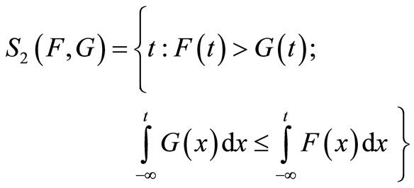
for all . Assume that this inequality holds for most of the range S, but not for all of it. Denote the area of SSD violation by:
 (4)
(4)
and denote the complement area of S2 by  (i.e.
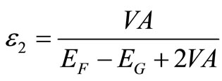
(i.e.  ). Define ε2 as the ratio:
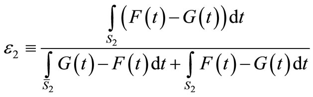 (5)
(5)
For ε2 < 0.5 F is said to “ε2-Almost SSD dominate” G. If F ε2-Almost SSD dominates G then EFu ≥ EGu for all preferences , where
  is the set of all “reasonable” risk-averse utility functions given by:
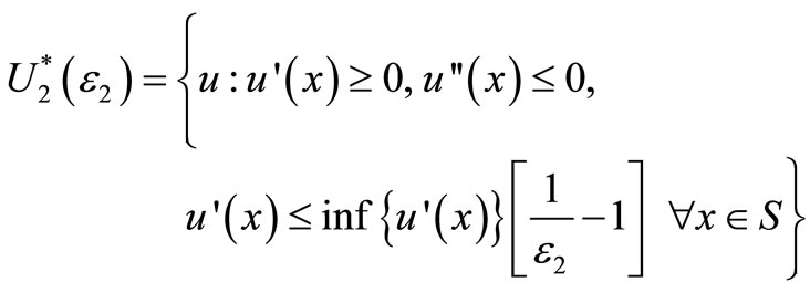 (6)
(6)
For ε2 = 0  is the set of all non-decreasing concave preferences and ASSD reduces to the standard SSD criterion. For proof of the ASD criteria and more detail, see [1,27]9.
3. ASD Algorithms
For FSD, SSD, and MV there are well-known algorithms for constructing the efficient sets. However, for AFSD and ASSD such algorithms have not yet been developed, and therefore, the effectiveness of these novel investment criteria has not yet been tested. Below we construct algorithms for obtaining the AFSD and ASSD efficient sets. In the next section we employ these algorithms to derive the empirical efficient ASD sets, and to compare them with the standard SD efficient sets.
3.1. AFSD Algorithm
The algorithms for constructing the empirical ASD efficient sets are based on pair-wise comparisons of all the different investments. If an investment is ASD dominated by some other investment, it is excluded from the efficient set. If it is not dominated by any other investment, it is included in the efficient set10. Generally, empirical studies rely on historical return observations, e.g. a set of n annual or monthly returns on various assets. Suppose that we want to compare two investments, F and G, each with n return observations. Denote the observations by xi and yi, corresponding to F and G, respectively (i = 1, 2, ···, n). Assume, without loss of generality, that the observations are ordered such that: x1 ≤ x2 ≤ ··· ≤ xn and y1 ≤ y2 ≤ ··· ≤ yn.
The total area between the cumulative distributions F and G is given by: 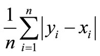 .
.
The area of violation of the FSD dominance of F over G is given by 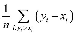
(see Figure 2(a) and Leshno and Levy [1]). Thus, the relative area violation is given by:
 . (7)
. (7)
Recall that ε1 is the actual area violation for F and G.
 (a) F AFSD Dominates G with
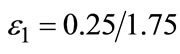
 (b) F ASSD Dominates G with
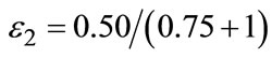
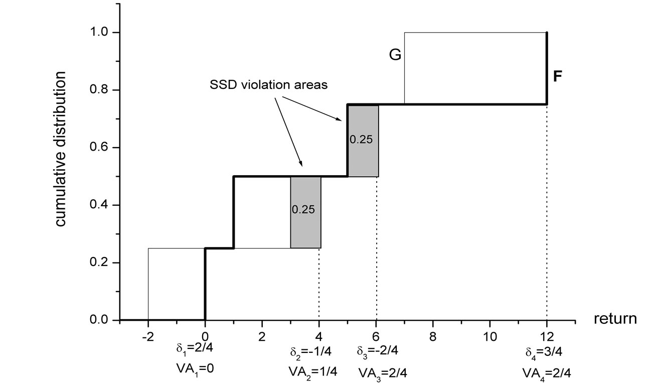
Figure 2. AFSD and ASSD-violation areas. (a) The total area enclosed between the two cumulative distributions is , in this case:
 . The violation area is the area where F > G, in this case 0.25. ε1 is given by the ratio 0.25/1.75. (b) The violation areas are the shaded areas (see Equation (4)). i = 2 demonstrates the case where a violation “block” follows a non-violation block, and the contribution to the violation area, is simply
  (second case in the ASSD algorithm). i = 3 demonstrates the case where a violation “block” follows a preceding violation block, and the contribution to the violation area is
 . It is simply the area of the new violation block (this is the third case in the ASSD algorithm). We have VA = 0.5, EF – EG = 0.75, and
 .
.
Thus, if we are considering the AFSD efficient set with some ε, then if ε1 ≤ ε, F will exclude G from the efficient set, but if ε1 > ε, it will not.
3.2. ASSD Algorithm
Note that ε2 can be written as follows:
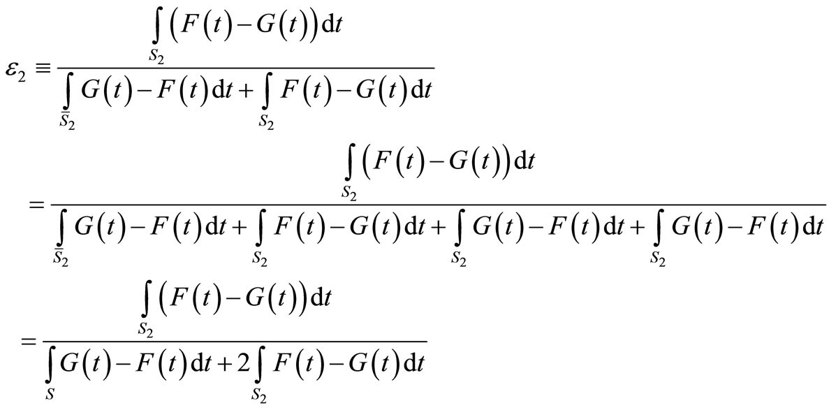
where the last equality stems from the fact that
(because ), and the fact that
 .
.
Recall that
 where EF and EG denote the mean returns of F and G (see [8]). Finally, let us denote the SSD violation area in short by VA,
to obtain:
 .11(8)
The ASSD algorithm is composed of the following steps:
1) Calculate the mean returns:
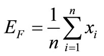 ,
,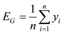 .
.
2) For all i: 1, 2, ···, n define
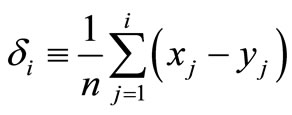 .
.
Every pair of return observations (xi, yi) adds a “block” of height  to the area enclosed between the two cumulative distributions. δi is the area between the two cumulative distributions up to the i’th observation, where the range in which G > F makes a positive contribution to the area, and the range in which F > G makes a negative contribution, see Figure 2(b). Define δ0 = 0.
3) Define by VAi the total area violation up to the ith observation. Define VA0 = 0. The total area violation for the entire distributions, VA in Equation (8), is given by VA = VAn.
4) For every i: 1, 2, ··· n:
o if δi ≥ 0: VAi = VAi–1 (there is no SSD violation and therefore there is no contribution to the SSD violation area. See, for example, the cases i = 1 and i = 4 in Figure 2(b)).
o if δi < 0 and δi–1 ≥ 0 (i.e., this is an area of violation, following a block of no violation): VAi = VAi–1 + . (See, for example, the case i = 2 in Figure 2(b)).
o if δi < 0 and δi–1 < 0 (i.e., this is an area of violation, following a previous block of violation): 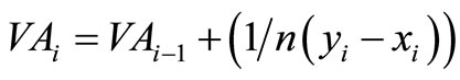 (See, for example, the case i = 3 in Figure 2(b)).
Figure 2(b) illustrates these three different cases (note that the second and third cases are different—if we had applied VAi = VAi–1 +  in the third case we would have double-counted the previous violation area δi–1, see Figure 2(b)).
5) VA = VAn. Plug VA, EF, and EG into Equation (8) to obtain the relative are violation, ε2.
A Matlab program for deriving the AFSD and ASSD efficient sets for any number of investments and any desired level of ε is available from the author upon request. For 100 assets and 50 return observations the program constructs the ASD efficient sets within a matter of seconds.
4. Empirical Results
4.1. The ASD Efficient Sets
To investigate the magnitude of the reduction of the efficient sets achieved by employing ASD instead of the standard SD, we perform the following analysis. As our investment universe we take the Fama-French 100 portfolios formed on size and book-to-market, with annual returns in the period 1956-2005 (for more details on the construction of these portfolios, and for the data itself, see Ken French’s website: http://mba.tuck.dartmouth.edu/pages/faculty/ken.french/data_library-.html). We first construct the standard MV, FSD, and SSD efficient sets, employing the standard algorithms in the literature (see, for example, Levy 2006). Next, we employ the algorithms developed in Section 3 to construct the AFSD and ASSD efficient sets for various levels of ε. We should stress that the results are not sensitive to the sample employed: similar results are obtained for other assets and sample periods.
Figure 3 illustrates one empirical comparison. The figure shows the cumulative return distributions of two portfolios in the FSD efficient set: portfolio 96, which is the portfolio with the lowest variance of all of the 100 Fama-French portfolios, and portfolio 29 (portfolio 96 is in the largest stock decile, with medium book-to-market; portfolio 29 is in the third smallest stock decile with high book-to-market). Note that portfolio 29 does not dominate portfolio 96 by FSD, because of a small FSD area violation around a return value of –20%, where P29 > P96 and P29 and P96 denote the respective cumulative return distributions (see Figure 3). However, the relative area violation is very small, and P29 ε-AFSD dominates P96 for ε = 0.01. Thus, P96 is in the FSD efficient set, however, it is not in the AFSD efficient set for ε ≥ 0.01. Indeed, looking at the cumulative return distributions it is evident that the preferences that assign higher expected utility to P96 than to P29 have to be quite extreme.
The FSD, MV, and SSD efficient sets contain 74, 13and 9 of the 100 portfolios, respectively. These sizes of the efficient sets (as a proportion of the total number of investments) are quite typical of the results in the literature obtained for other sets of assets. The sizes of the AFSD and ASSD efficient sets as a function of ε are shown in Figure 4. Note that the standard FSD and SSD sets correspond to the AFSD and ASSD for the special case of ε = 0 (i.e. no violation whatsoever is allowed). The AFSD and ASSD efficient sets decrease rather dramatically as ε increases.
An important question is what is a reasonable value of ε to employ? Levy, Leshno and Leibovich [26] experimentally estimate the relevant value as ε = 0.06. They find that if the area violation is smaller than this value, all subjects in their experiments choose the ASD dominating investment. With this experimental value, the reduction in the efficient sets is significant: The AFSD efficient set contains only 27 portfolios (a reduction of 64% relative to the 74 portfolios in the FSD efficient set), and the ASSD efficient set contains 7 portfolios (a reduction of 22% relative to the 9 portfolios in the SSD efficient set, see Figure 4).
Levy, Leshno and Leibovich experimentally find ε = 0.06. Hence, they exclude some preferences considered “unreasonable” as they do not characterize any of the subjects in their experiments. It is interesting to find the range of preference parameters corresponding to this area violation value. In other words, how “crazy” does the utility function have to be for portfolios outside of the ASD efficient set to be selected? To this question we turn next.
4.2. Direct Expected Utility Analysis
The portfolios excluded from the ASD efficient sets
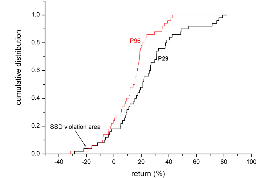
Figure 3. Empirical example. Both portfolios are in the FSD efficient set. Portfolio P29 does not dominate portfolio P96 because there is a small area of FSD violation where P29 > P96. However, P29 ε-AFSD dominates P96 with ε = 0.01.
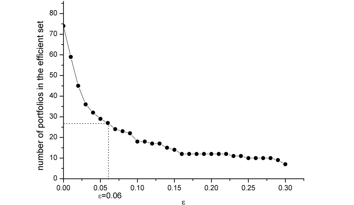 (a) AFSD Efficient Set-100 FF Portfolios
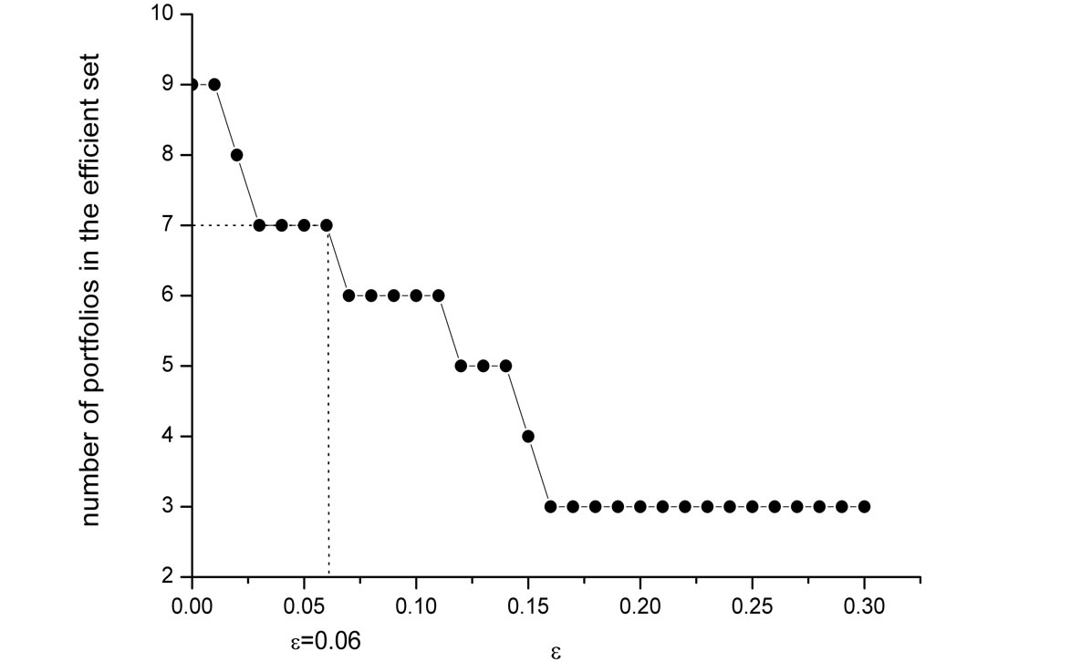 (b) ASSD Efficient Set-100 FF Portfolios
 Figure 4: Empirical AFSD and ASSD efficient sets. The set of investments is the Fama-French universe of 100 portfolios formed on size and book-to-market. (a) Shows the AFSD efficient set as a function of the allowed violation ε; (b) Shows the ASSD efficient set. ε = 0 corresponds to the standard FSD and SSD efficient sets. For the experimentally estimated value of ε = 0.06, the AFSD efficient set contains only 27 portfolios, and the ASSD efficient set contains only 7 portfolios.
could, in principle, be the optimal portfolios for some EU maximizers. The experimental results of [26] suggest that in practice individuals with these preferences are very hard to find. In order to shed more light on this issue, we ask the following question: we look at the AFSD efficient set with ε = 0.06, and we ask what preferences will imply a choice of investments outside of this AFSD efficient set. We focus on the AFSD efficient set because we will consider different preference classes, some of which are not risk averse (Prospect Theory preferences).
We first consider investors with CRRA preferences:
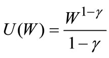 .
.
The relative risk aversion coefficient, γ, is typically estimated in the range 1 - 3 (see, for example, [29]). In our analysis we consider a much wider range: we take γ in the huge range 1 ≤ γ ≤ 100. For each value of γ (with increments of 0.01) we numerically find the optimal investment (by direct EU calculation for all the 100 portfolios), and we check whether this portfolio is in or out of the AFSD efficient set. We find that the optimal portfolios for all preferences in the range 1≤ γ ≤ 100 are included in the AFSD efficient set. Thus, we find that no individual with conceivable CRRA preferences chooses any investment outside the AFSD efficient set. We repeat this analysis for other standard preferences. For CARA preferences of the form
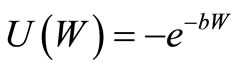
We find that no investor with parameters in the range 0 ≤ bW0 ≤ 500, where W0 is the initial wealth, chooses any investment outside the AFSD efficient set.
We also examine the case of the non-risk-averse Prospect Theory preferences suggested by Tversky and Kahneman [30]:
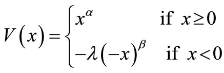
where x is the change in wealth relative to the current wealth, and α, β and λ are constants experimentally estimated as: α = 0.88, β = 0.88, λ = 2.25. The investor’s optimal investment is determined by the maximization of E[V(x)]12. We find the optimal investment for preferences with loss aversion in the very wide range of 1 ≤ λ ≤ 10. Again, we find that all choices fall within the AFSD efficient set with ε = 0.06. Thus, it seems that the reduction of the efficient set comes at very little cost in terms of excluding investments that would have been chosen by any reasonable investors.
5. Conclusion
Empirical and experimental results suggest that the standard SD and MV efficient sets include a large number of investments that are very unlikely to be chosen by any real-world investor. Almost FSD (AFSD) and Almost SSD (ASSD) are new criteria that allow us to eliminate such investments from the efficient sets, by excluding very unrealistic preferences that are considered “pathological”.
In this study we employ MV, SD, and ASD criteria with two purposes:
1) To find the reduction of the efficient sets obtained with the ASD criteria.
2) To examine whether the preferences excluded by ASD are indeed unrealistic.
The algorithms developed in this paper are used to derive the AFSD and ASSD efficient sets. The reduction of the efficient sets obtained by ASD is significant: for the set of 100 Fama-French portfolios formed on size and book-to-market we find that the AFSD efficient set with ε = 0.06 includes only 27 portfolios (relative to the 74 portfolios in the standard FSD efficient set), and the ASSD efficient set includes only 7 portfolios (relative to the 9 portfolios in the standard SSD efficient set).
Experimental evidence and direct EU maximization suggest that this improvement comes at very little cost in the sense of excluding portfolios that would have been chosen by any real-world investors. To be more specific, we examine three commonly-employed preference families and we find that the excluded preferences are characterized by very extreme parameter values. Thus, it seems justified to exclude these preferences from the set of preferences relevant for economic decision-making.
REFERENCES
- M. Leshno and H. Levy, “Preferred by ‘All’ and Preferred by ‘Most’ Decision Makers: Almost Stochastic Dominance,” Management Science, Vol. 48, No. 8, 2002, pp. 1074-1085. doi:10.1287/mnsc.48.8.1074.169
- G. Chamberlain, “A Characterization of the Distributions that Imply Mean-Variance Utility Functions,” Journal of Economic Theory, Vol. 29, No. 1, 1983, pp. 185-201. doi:10.1016/0022-0531(83)90129-1
- J. Owen and R. Rabinovitch, “On the Class of Elliptical Distributions and their Applications to Portfolio Choice,” Journal of Finance, Vol. 38, No. 3, 1983, pp. 745-752. doi:10.1111/j.1540-6261.1983.tb02499.x
- J. Berk, “Necessary Conditions for the CAPM,” Journal of Economic Theory, Vol. 73, No. 1, 1997, pp. 245-257. doi:10.1006/jeth.1996.2218
- H. Levy and H. Markowitz, “Approximating Expected Utility by a Function of Mean and Variance,” American Economic Review, Vol. 69, No. 3, 1979, pp. 308-317.
- H. Markowitz, “Foundations of Portfolio Theory,” Journal of Finance, Vol. 46, No. 2, 1991, pp. 469-477. doi:10.1111/j.1540-6261.1991.tb02669.x
- J. Hadar and W. Russell, “Rules for Ordering Uncertain Prospects,” American Economic Review, Vol. 59, No. 1, 1969, pp. 25-34.
- G. Hanoch and H. Levy, “The Efficiency Analysis of Choices Involving Risk,” Review of Economic Studies, Vol. 36, 1969, pp. 335-346. doi:10.2307/2296431
- M. Rothschild and J. Stiglitz, “Increasing Risk: I. A Definition,” Journal of Economic Theory, Vol. 2, No. 3, 1970, pp. 225-243. doi:10.1016/0022-0531(70)90038-4
- E. De Giorgi, “Reward-Risk Portfolio Selection and Stochastic Dominance,” Journal of Banking and Finance, Vol. 29, No. 4, 2005, pp. 895-926. doi:10.1016/j.jbankfin.2004.05.027
- D. Dentcheva and A. Ruszczynski, “Portfolio Optimization with Stochastic Dominance Constraints,” Journal of Banking and Finance, Vol. 30, No. 2, 2006, pp. 433-451. doi:10.1016/j.jbankfin.2005.04.024
- G. Constantinides and S. Perrakis, “Stochastic Dominance Bounds on American Option Prices in Markets with Frictions,” Review of Finance, Vol. 11, No. 1, 2007, pp. 71-116. doi:10.1093/rof/rfl001
- D. Gasbarro, W. Wong and J.K. Zumwalt, “Stochastic Dominance Analysis of iShares,” European Journal of Finance, Vol. 13, No. 1, 2007, pp. 89-101. doi:10.1080/13518470601025243
- W. K. Wong, “Stochastic Dominance and Mean-Variance Measures of Profit and Loss for Business Planning and Investment,” European Journal of Operational Research, Vol. 182, No. 2, 2007, pp. 829-843. doi:10.1016/j.ejor.2006.09.032
- A. Abhyankar, K. Y. Ho and H. Zhao, “Value versus Growth: Stochastic Dominance Criteria,” Quantitative Finance, Vol. 8, No. 7, 2008, pp. 693-704. doi:10.1080/14697680701668426
- J. Annaert, S. Van Osselaer and B. Verstraete, “Performance Evaluation of Portfolio Insurance Strategies Using Stochastic Dominance Criteria,” Journal of Banking and Finance, Vol. 33, No. 2, 2009, pp. 272-280. doi:10.1016/j.jbankfin.2008.08.002
- M. Kopa and T. Post, “A Portfolio Optimality Test Based on the First-Order Stochastic Dominance Criterion,” Journal of Financial and Quantitative Analysis, Vol. 44, No. 5, 2009, pp. 1103-1124. doi:10.1017/S0022109009990251
- H. Levy, “Stochastic Dominance: Investment Decision Making Under Uncertainty,” Springer, New York, 2006.
- H. Zhang, W. Song, X. Peng and X. Song, “Evaluate the Investment Efficiency by Using Data Envelopment Analysis: The Case of China,” American Journal of Operations Research, Vol. 2 No. 2, 2012, pp. 174-182.
- R. B. Porter and J. E. Gaumnitz, “Stochastic Dominance vs. Mean Variance Portfolio Analysis: An Empirical Evaluation,” American Economic Review, Vol. 62, No. 3, 1972, pp. 438-446.
- H. Tehranian, “Empirical Studies in Portfolio Performance Using Higher Degrees of Stochastic Dominance,” Journal of Finance, Vol. 35, No. 1, 1980, pp. 159-171. doi:10.1111/j.1540-6261.1980.tb03478.x
- V. S. Bawa, J. Bondurtha, M. R. Rao and H. L. Suri, “On Determination of the Stochastic Dominance Optimal Set,” Journal of Finance, Vol. 40, No. 2, 1985, pp. 417-431. doi:10.1111/j.1540-6261.1985.tb04965.x
- M. Levy, “Are Rich People Smarter?” Journal of Economic Theory, Vol. 110, No. 1, 2003, pp. 42-64. doi:10.1016/S0022-0531(03)00024-3
- P. C. Benitez, T. Kuosmanen, R. Olschewski and G. C. van Kooten, “Conservation Payments Under Risk: A Stochastic Dominance Approach,” American Journal of Agricultural Economics, Vol. 88, No. 1, 2006, pp. 1-15. doi:10.1111/j.1467-8276.2006.00835.x
- J. Huang, “Almost First Stochastic Dominance: What Do We Know from the Options Market?” SSRN Working Paper, 2007.
- H. Levy, M. Leshno and B. Leibovich, “Economically Relevant Preferences for All Observed Epsilon,” Annals of Operations Research, Vol. 176, No. 1, 2010, pp. 153- 178. doi:10.1007/s10479-008-0470-7
- M. Levy, “Almost Stochastic Dominance and Stocks for the Long Run,” European Journal of Operations Research, Vol. 194, No. 1, 2009, pp. 250-257. doi:10.1016/j.ejor.2007.12.017
- P. C. Fishburn, “Convex Stochastic Dominance with Continuous Distributions,” Journal of Economic Theory, Vol. 7, No. 2, 1974, pp. 143-158. doi:10.1016/0022-0531(74)90103-3
- I. Friend and M. Blume, “The Demand for Risky Assets,” American Economic Review, Vol. 65, No. 5, 1975, pp. 900-922.
- A. Tversky and D. Kahneman, “Advances in Prospect Theory,” Journal of Risk and Uncertainty, Vol. 5, No. 4, 1992, pp. 297-323. doi:10.1007/BF00122574
NOTES
1Or, more generally, in the case of elliptical distributions [2-4]. MV is also a sufficient but not a necessary rule for quadratic preferences.
2The Stochastic Dominance criteria were developed independently by Hadar and Russell [7], Hanoch and Levy [8], and Rothschild and Stiglitz [9]. Literally hundreds of papers have been written on the theory and application of Stochastic Dominance to financial decisionmaking. For some recent examples, see [10-17]. For a comprehensive review of SD see Levy [18]. Data Envelopment Analysis is an alternative approach to investment efficiency analysis [19].
3See, for example [20-22].
4Obviously, the more assumption made regarding preferences, the smaller the efficient set (hence the TSD efficient set is a subset of the SSD efficient set, which is a subset of the FSD efficient set), where TSD stands for Third degree SD, SSD stands for Second degree SD, and FSD stands for First degree SD.
5The cumulative distributions of F and G intersect (see Figure 1), thus, there is no FSD dominance. There is no SSD dominance either, because the minimal outcome of F is lower than the minimal outcome of G (for a formal definition, see the SSD integral condition below).
6SD criteria are based on pairwise comparisons of the investments under consideration. Recently, the scope of SD has been extended to allow examination of portfolios of the underlying investments. Namely, given a set of assets, one can ask whether a specific portfolio of these assets is in the SD efficient set. The problem of SD illustrated by the example in the text also holds in the portfolio framework, all portfolios of F and G in the above example are in the SD efficient set, even though most of these portfolios wouldn’t be chosen by any “reasonable” investor.
7AMV is a special case of ASD when the return distributions are normal (just as MV coincides with SD for normal distributions). Here we analyze the more general ASD criterion, without restricting the discussion to the case of normal distributions.
8Levy [23] investigates the distribution of wealth at the high wealth range, and employs Almost Stochastic Dominance to develop a simple stochastic model that can explain the empirically observed power-law wealth distribution. Benitez, Kuosmanen, Olschewski, and van Kooten [24] use Almost Stochastic Dominance to determine the minimal conservation payments required to guarantee that the environmentallypreferred use of land dominates other less environmentally-preferred alternatives. Gasbarro, Wong, and Zumwalt [13] employ Almost Stochastic Dominating in ranking 18 country market indices. Huang [25] employs Almost Stochastic Dominance to derive bounds on the prices of various options. Levy, Leshno and Leibovich [26] investigate ASD experimentally.
9[1] and [27] provide two alternative formulations of ASSD. Here we employ Levy’s [27] formulation, which is more straightforward. Levy [27] employs integration by parts and the fact that u(x) is concave to prove that if 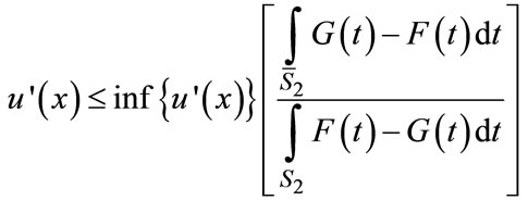 for all
 , then EUF > EUG [see Equations (13.12), p. 342). Using the definition of ε2 in Equation (5) and a little algebraic manipulation, the above condition can be written as the dominance condition in (6):
  .
.
10One can further reduce the efficient set by employing higher dimensional comparisons, i.e. Convex SD (see Fishburn [28]). Here we employ the standard pair-wise methodology, and compare it with the standard SD pair-wise methodology. The development of Convex ASD criteria seems like a promising research avenue, but it is beyond the scope of this paper.
11It is interesting to note that Equation (8) implies that having a greater (or equal) mean return is a necessary condition for ε-ASSD: if EF < EG by (8) we have ε2 > 0.5, i.e. F does not dominate G by ε-ASSD.
12Another element of Prospect Theory is that of subjective probability weighting. As it is not clear if subjective weighting occurs in the present case where all outcomes are equally likely, and as this element is foreign to the preference considerations discussed here, we abstract away from this element.