American Journal of Operations Research
Vol. 2 No. 1 (2012) , Article ID: 17829 , 8 pages DOI:10.4236/ajor.2012.21006
Optimal Policy for EOQ Model with Two Level of Trade Credits in One Replenishment Cycle
1Department of Mathematics and Humanities, Sardar Vallabhbhai National Institute of Technology (SVNIT), Surat, India
2Department of Mathematics, Dev Nagri (Post Graduate) College, Meerut, India
3Department of Mathematics, PDM College of Engineering, Bahadurgarh, India
Email: {amitsharmajrf, dr.ruchigoel}@gmail.com, ndua_10@yahoo.com
Received October 21, 2011; revised November 28, 2011; accepted December 8, 2011
Keywords: EOQ Model; Inventory; Two Levels of Trade Credit; Replenishment Cycle
ABSTRACT
In general, a supplier/retailer frequently offer trade credit to stimulate their respective sales. The main purpose of this paper is to investigate the optimal supplier/retailer’s replenishment decisions under two levels of trade credit policy within the economic order quantity (EOQ) framework. This paper deals with the supplier/retailer’s inventory replenishment problem under two levels of trade credit in one replenishment cycle. A different approach of two levels of trade credit is used, which give more freedom to the supplier/retailer in business. In addition, the easy-to-use procedure is developed to efficiently find the optimal cycle time for the retailer under minimizing annual total relevant cost. Finally, a numerical example is given to illustrate these results.
1. Introduction
The traditional economic order quantity (EOQ) model is widely used by practitioners as a decision-making tool for the control of inventory. It was tacitly assumed that the buyer must pay for the items purchased as soon as the items are received. However, in practice, the supplier frequently offers the trade credit (or permissible delay in payments) to attract retailer who considers it to be a type of price reduction. Trade credit has long been a subject of interest to financial economists. At the theoretical level, various explanations have been offered to account for the optimal choice of trade credit made by supplier/retailer. The empirical research has followed this lead, examining in detail the cross-sectional determinants of trade credit among supplier/retailer.
Sometimes supplier/retailer’s can’t pay at the given credit period and at this stage they paid the higher interest, but in our model, a different approach of two levels of trade credit is used. In this approach, the account is settled at two times in one replenishment cycle. The interest charge, when the account is settled at first time is lesser than the interest charge, when the account is settled at second time in a cycle. In this model, supplier/ retailer has the opportunity to pay within second credit period. So that, they can increase the sales revenue and reduced their total cost to earn the interest within credit period. But after that they have to pay a higher interest. In this approach, the customer will be attracted and the sales will be increased.
Chung [1] developed an alternative approach to determine the economic order quantity under condition of permissible delay in payments. Recently, Huang [2] modified this assumption to two levels of trade credit, that is, not only the supplier offers its retailer the trade credit but also the retailer offers its customer the trade credit. But the decay item was ignored in their models. Chung and Liao [3] deal with the problem of determining the economic order quantity for exponentially deteriorating items under permissible delay in payments depending on the ordering quantity. Jamal et al. [4] developed an ordering policy with trade credit. In their model shortages are allowed. Chang and Dye [5] gave an article for deteriorating items with partial backlogging and permissible delay in payments. Huang and Liao [6] discussed a simple method to locate the optimal solution for exponentially deteriorating items when the supplier permits not only a cash discount but also a permissible delay. Kreng and Tan [7] discussed the optimal replenishment decisions under two levels of trade credit policy depending on the order quantity. Ouyang et al. [8] proposed an optimal policy for non-instantaneous deteriorating items when the supplier provides permissible delay in payments. Hou and Lin [9] developed a cash flow oriented EOQ model with deteriorating items under permissible delay in payments and the minimum total present value of the costs is obtained. In this paper all results have been obtained by taking constant net discount rate of inflation k. He obtained minimum total present value of the costs over the time horizon.
Trade credit is a marketing strategy to increase sales and reduce inventories. Therefore, optimal inventory policies that consider both the supplier and customer viewpoints are more reasonable than those that consider only from one perspective. Therefore, this study develops an inventory model with two levels of trade credit in one replenishment cycle. Moreover, an easy-to-use algorithm with cost minimization is provided to obtain the optimal number of replenishment, cycle time and order quantity. Finally, a numerical example is presented to illustrate the theoretical results for the cases given below:
Case I: M ≤ T, The credit period is less than or equal to the cycle time T for settling the account, where M is the permissible delay in payment when the account is settled at first time.
Case II: M > T, The credit period is greater than the cycle time for settling the account.
Case III: M < N ≤ T, The credit period is less than or equal to the cycle time T for settling the account, where N is the permissible delay in payment when the account is settled at second time.
Case IV: M < T < N, The credit period is greater than the cycle time for settling the account.
2. Preliminaries
2.1. Notations
The following notations are used throughout the paper:
H length of planning horizon;
T replenishment cycle time;
n number of replenishment during the planning horizon, T = H/n;
Q order quantity, units/cycle;
A ordering cost at time zero, $/order;
c per unit cost of the item, $/unit;
h unit stock holding cost per item per year excluding interest charges;
θ deterioration rate, fraction of units that deteriorate per time unit;
M the permissible delay in payment in settling the account at first time;
N the permissible delay in payment in settling the account at second time;
 the interest earned per dollar per unit time;
 the interest charged per dollar in stocks per unit time, when M is the trade credit,
 ;
;
 the interest charged per dollar in stocks per unit time, when N is the trade credit,
 .
.
2.2. Assumptions
The mathematical model in this paper is developed with the following assumptions:
1) Demand rate, D, is known and constant;
2) Shortages are not allowed;
3) Replenishment is instantaneous;
4) There is no repair or replacement of the deteriorated inventory during a given cycle;
5) The constant fraction θ of on hand inventory gets deteriorated per time unit;
6) When M ≤ T, the account is settled at  and the supplier/retailer starts paying interest on the items in stock with the rate of interest Ic. When M > T, the account is settled at
  and the supplier/retailer does not need to pay any interest charge;
7) When M < N ≤ T, the account is settled at  and the supplier/retailer starts paying interest on the items in stock with the rate of interest Ic between M to N and Iw between N to T. When M < T < N, the account is settled at
  and the supplier/retailer starts paying for the interest charges on the items in stock with rate Ic.
3. Model Formulation
The total time horizon H has been divided into n equal parts of length T so that T = H/n. This model is illustrated in Figure 1.
Let  denote the on-hand inventory level at time t, which is depleted by the effects of demand and deterioration. There are n cycles and at
 ,
,  is the initial inventory and at
 , the inventory is finished, then the differential equation which describes the instantaneous states of
  over
over  is given as:
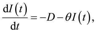 where
where  (1)
(1)
then, with boundary condition . The solution of above equation is given by
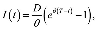 where
where  (2)
(2)
Noting that,  , the quantity ordered each replenishment cycle is
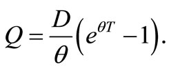 (3)
(3)
Since there are n replenishments in the entire horizon H, the present value of the total replenishment costs is given by
 (4)
(4)
and, the present value of deterioration costs is given by
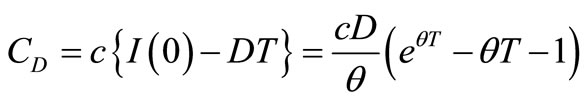 . (5)
. (5)
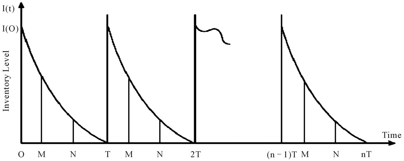
Figure 1. The graphical representation of inventory cycle.
The present value of the holding costs during the first replenishment cycle is
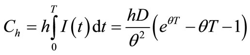 . (6)
. (6)
Trade credit is the process of “buy now, pay later”. Since the inventory model considers the effect of two level of trade credits, there are four distinct types of cases in inventory system.
Case I. 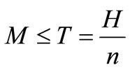
In this case, the trade credit period M is less than or equal to the replenishment cycle time T. Therefore, the delay in payments is permitted and the total relevant cost includes both the interest charged and the interest earned. The present value of the interest payable during the first replenishment cycle is
 . (7)
. (7)
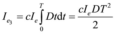
Next, the present value of the total interest earned during the first replenishment cycle is
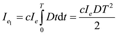 . (8)
. (8)
Case II. 
Since the trade credit period M is greater than to the replenishment cycle time T, so that the interest charged during the time period  is equal to zero, because the supplier/retailer can be paid in full at the permissible delay M. The interest earned during the time period
  plus the interest earned from the cash invested during the time period
  after the inventory is exhausted at time T, and is given by
 (9)
(9)
 . (10)
Case III. 
In this case, trade credit period N is less than or equal to the replenishment cycle time T, and is greater than to the trade credit period M. Therefore, the delay in payments is permitted and the total relevant cost includes both the interest charged and the interest earned. During this the interest charged is very high but the interest earned is same as-well-as the time of credit period M. At the period M to N the interest will be charged at the rate  and at the period N to T the interest will be charged at the rate
 , where
 . The present value of the interest payable during the first replenishment cycle is
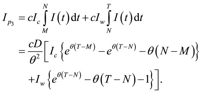 (11)
(11)
The present value of the total interest earned during the first replenishment cycle is
 . (12)
Case IV. 
In this case, trade credit period N is greater than to the replenishment cycle time T, and also greater than to the trade credit period M. Therefore, the interest charged with interest rate  during the time period
  is equal to zero, but the interest will be charged with interest rate
  during the time period
 . The present value of the interest payable during the first replenishment cycle is
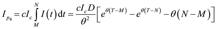 (13)
(13)
The interest earned during the time period  and the interest earned from the cash invested during the time period
  after the inventory is exhausted at time T. Thus, the present value of the total interest earned during the first replenishment cycle is
 . (14)
Since, there are n cycles in the planning horizon H, then the annual total relevant cost , which is a function of n, is given by
 = n [Replenishment cost + Deterioration cost
+ Holding cost + Interest paid – Interest earn]
i.e.
 (15)
(15)
Now, the total cost, when  is given by
 (16)
(16)
and, the total cost, when  is given by
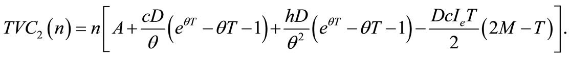 (17)
(17)
and, the total cost, when  is given by
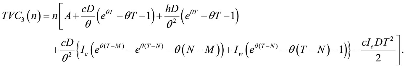 (18)
(18)
and, the total cost, when  is given by
 . (19)
According to the above arguments, we have
 (20)
(20)
where ,
,  ,
,  and
and  as expressed in Equations (16), (17), (18), and (19) respectively.
4. Algorithm
The following algorithm is developed to derive the optimal n, T, Q and  values:
Step 1: Choose a discrete variable n first, where n is any integer equal or greater than 1.
Step 2: If , for different integer n values, obtain
  from Equation (16); If
 , for different integer n values, obtain
  from Equation (17); If
 , for different integer n values, obtain
  from Equation (18); If
  , for different integer n values, obtain
  from Equation (19).
Step 3: Repeat step 1 and 2 for all possible values of n with  until the minimum
  is found from Equation (16) and let
 . For all possible values of n with
  until the minimum
is found from Equation (17) and let . For all possible values of n with
  until the minimum
  is found from Equation (18) and let
 . For all possible values of n with
 until the minimum
  is found from Equation (19) and let
 . The
. The ,
,  ,
,  ,
,  ,
,  ,
,  ,
,  , and
, and  values constitute the optimal solution.
Step 4: Select the optimal number of replenishment  such that
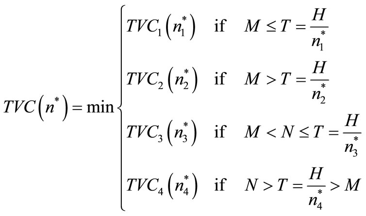 (21)
(21)
Thus, optimal order quantity  is obtained by putting
  into (3) and optimal cycle time
  is
is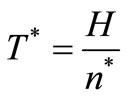 .
.
5. Numerical Example
To illustrate the results of the model developed in this study an example is given with the following data:
The demand rate, D = 960 unit/year, the replenishment cost, A = $60/order, the holding cost excluding interest charges, h = $1.5/unit/year, the per unit item cost, c = $ 3/unit, the deterioration rate, θ = 0.15, when account is settled at M, the interest charged per $ in stocks per year by the supplier/retailer, Ic = $0.18/$/year, the interest earned, Ie = $0.16/$/year, when account is settled at N, the interest charged per $ in stocks per year by the supplier/retailer, Iw = $0.21/$/year, and the planning horizon, H = 5 year. The delay in payment in settling account, M = 0.083 year, and N = 0.14 year, assuming 360 days per year. Using the algorithm, we have the computational results shown in Table 1.
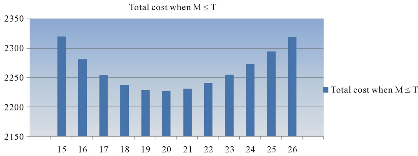
The graphical representation of total cost when M ≤ T, M > T, M < N ≤ T and N > T > M are given in Figures 2(a)-(d) respectively which are given below.
In the numerical example, we see that the case I is optimal option in credit policy when the account is settled at “M”. The minimum total present value of costs is obtained when the number of replenishment, n, is 20. With 20 replenishments, the optimal (minimum) cycle time is 0.250 year, the optimal (minimum) order quantity, Q = 244.500 units and the optimal (minimum) total present value of costs,  = $2226.5765. Also, the case III is optimal option in credit policy when the account is settled at “N”. The minimum total present value of costs is obtained when the number of replenishment, n, is 20.
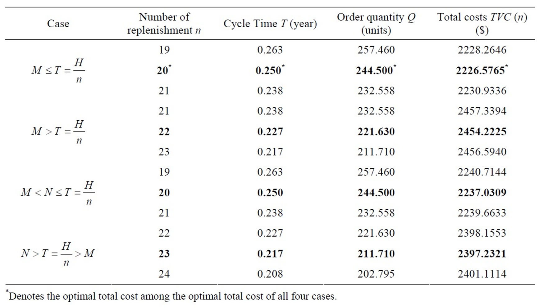
Table 1. Computational analysis for optimal total cost.
 (a)
(a)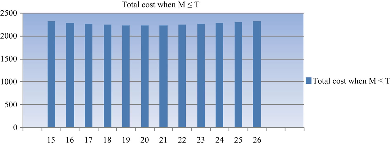 (b)
(b)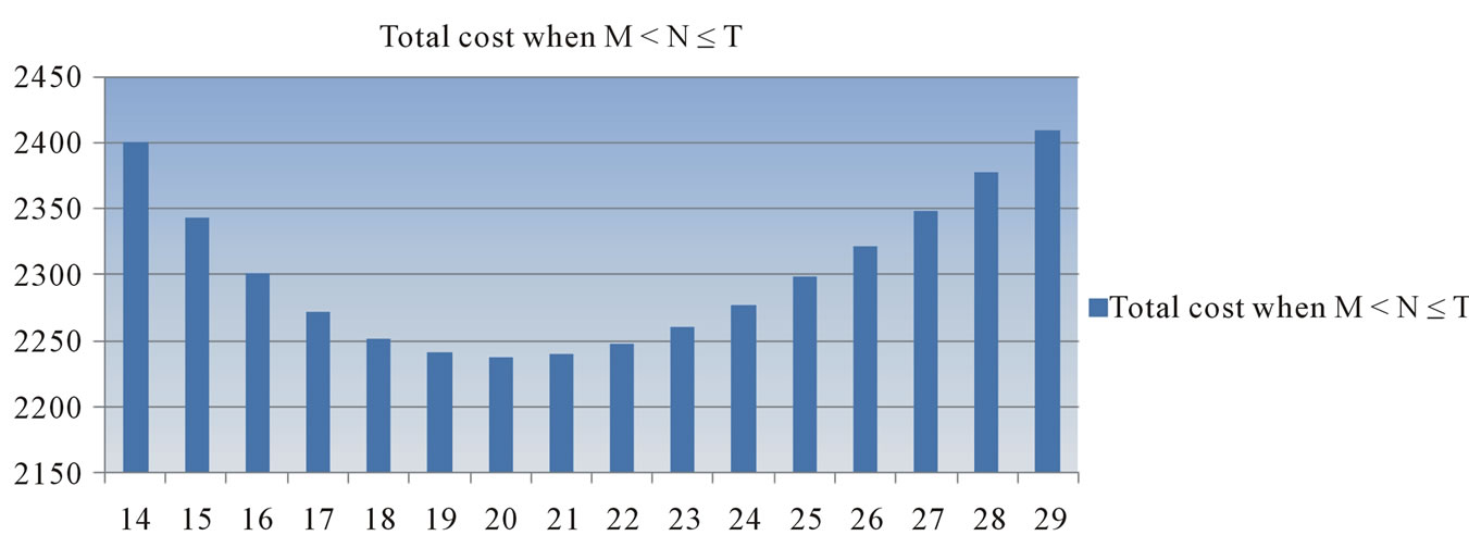 (c)
(c)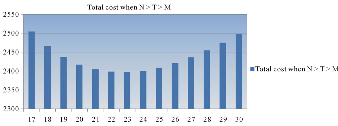 (d)
(d)
Figure 2. Plot of “n” against TVC (n).
With 20 replenishments, the optimal (minimum) cycle time is 0.250 year, the optimal (minimum) order quantity, Q = 244.500 units and the optimal (minimum) total present value of costs,  = $2237.0309.
In the total optimal cost, we see that, there is miner difference between the costs when the account is settled at “M” and at “N”. Thus, the model is more realistic to the business environment and gives more freedom to the suppliers/retailers to run business smoothly. By this policy, they can attract the customers and increase their sales. Therefore, the policy involves inventory, financing and marketing issue. So, we investigate that this model is very important and valuable to the enterprises.
6. Sensitivity Analysis
Taking all the parameters as in the above numerical example, the variation of the optimal solution for different values of M is given in Table 2, and variation of the optimal solution for different values of θ is given in Table 3.
The data obtained clearly shows those individual optimal solutions different from each other for different values of trade credit M, and the deterioration rate θ. All the observations can be summed up as follows:
1) In the total four cases,  ,
,  ,
,
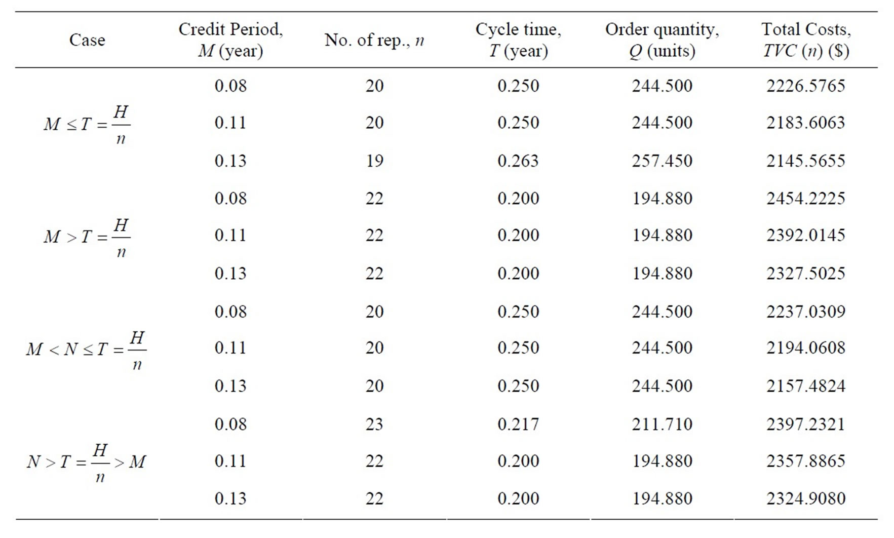
Table 2. Sensitivity analysis on M.
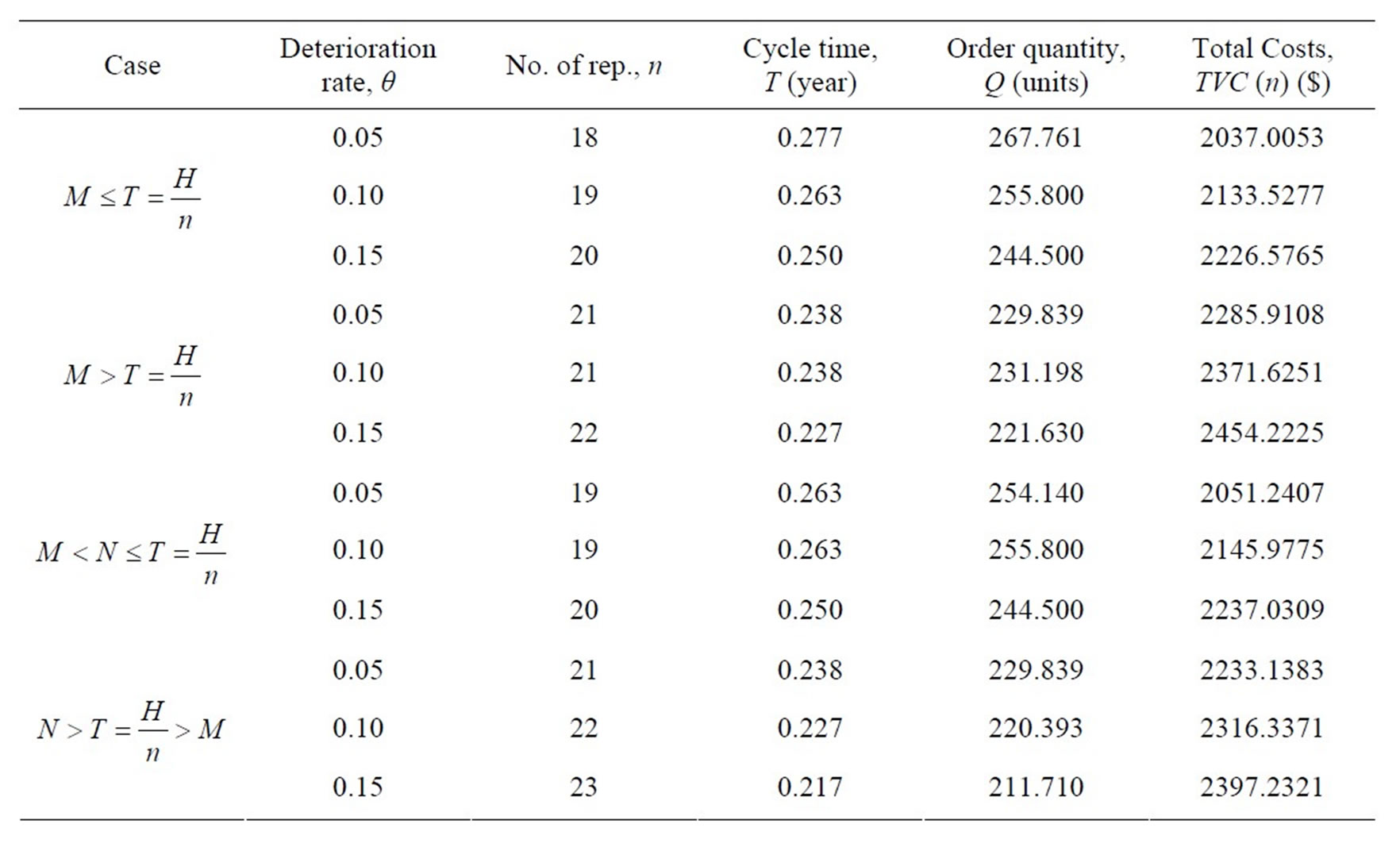
Table 3. Sensitivity analysis on θ.
 and
and , an increase in the trade credit M, the total costs are in decreasing trend.
2) Observed in Table 3, when deterioration rate (θ) increases then in the total four cases,  ,
,  ,
,  and
and , the total costs are in increasing trend.
7. Conclusion and Future Research
This study develops an inventory model for deteriorating items over a finite planning horizon, when the suppliers/ retailers provide two levels of permissible delay in payments in one replenishment cycle. The model considers the effects of permissible delay in payments at both stages. In addition, an optimal solution procedure is obtained to find the optimal number of replenishment, cycle time, and order quantity to minimize the total present value of cost. The proposed model can be extended in several ways, such as for time dependent demand and deterioration. The inflation rate may also be introduced. Finally, further research can be done with stochastic market demand and partial backlogging.
8. Acknowledgements
The first author is grateful to the CSIR, New Delhi for providing the financial assistance as JRF.
REFERENCES
- K. J. Chung, “A Theorem on the Determination of Economic Order Quantity under Conditions of Permissible Delay in Payments,” Computers & Operations Research, Vol. 25, 1998, pp. 49-52.
- Y. F. Huang, “Optimal Retailer’s Ordering Policies in the EOQ Model under Trade Credit Financing,” Journal of Operational Research Society, Vol. 54, No. 9, 2003, pp. 1011-1015. doi:10.1057/palgrave.jors.2601588
- K. J. Chung and J. J. Liao, “Lot-Sizing Decisions under Trade Credit Depending on the Ordering Quantity,” Computers & Operations Research, Vol. 31, No. 6, 2004, pp. 909-928. doi:10.1016/S0305-0548(03)00043-1
- A. Jamal, B. Sarker and S. Wang, “An Ordering Policy for Deteriorating Items with Allowable Shortage and Permissible Delay in Payment,” Journal of Operational Research Society, Vol. 48, No. 8, 1997, pp. 826-833.
- H. J. Chang and C. Y. Dye, “An Inventory Model for Deteriorating Items with Partial Backlogging and Permissible Delay in Payments,” Journal of Systems Science, Vol. 32, No. 3, 2001, pp. 345-352. doi:10.1080/002077201300029700
- K. N. Huang and J. J. Liao, “A Simple Method to Locate the Optimal Solution for Exponentially Deteriorating Items under Trade Credit Financing,” Computers and Mathematics with Applications, Vol. 56, No. 4, 2008, pp. 965-977. doi:10.1016/j.camwa.2007.08.049
- V. B. Kreng and S. J. Tan, “The Optimal Replenishment Decisions under Two Levels of Trade Credit Policy Depending on the Order Quantity,” Expert Systems with Applications, Vol. 37, No. 7, 2010, pp. 5514-5522. doi:10.1016/j.eswa.2009.12.014
- L. Y. Ouyang, K. S. Wu and C. T. Yang, “A Study on an Inventory Model for Non-Instantaneous Deteriorating Items with Permissible Delay in Payments,” Computers and Industrial Engineering, Vol. 51, No. 4, 2006, pp. 637-651. doi:10.1016/j.cie.2006.07.012
- K. L. Hou and L. C. Lin, “A Cash Flow Oriented EOQ Model with Deteriorating Items under Permissible Delay in Payments,” Journal of Applied Sciences, Vol. 9, No. 9, 2009, pp. 1791-1794. doi:10.3923/jas.2009.1791.1794