Journal of Environmental Protection, 2011, 2, 564-570
doi:10.4236/jep.2011.25065 Published Online July 2011 (http://www.scirp.org/journal/jep)
Optimizing Non-Ferrous Metal Value from MSWI
Bottom Ashes
Simon P. M. Berkhout1, Bert P. M. Oudenhoven2, Peter C. Rem1
1Delft University of Technology, Delft, the Netherlands; 2Twence Afval en energie, Hengelo, the Netherlands.
Received March 22nd, 2011; revised April 28th, 2011; accepted June 1st, 2011.
ABSTRACT
The bottom ashes resulted annually from the incineration of municipal solid waste in Europe contain about 400,000
tonnes of metallic aluminium and 200,000 tonnes of heavy non-ferrous metals, such as copper and zinc. Efficient re-
covery of this non-ferrous metal resource requires state-of-the-art separation technologies and a continuous feedback
of laboratory analyses of the metal products and the depleted bottom ash to the operators of the bottom ash treatment
plants. A methodology is presented for the optimization of the production of non-ferrous metal value from Municipal
Solid Waste Incinerator bottom ash. Results for an incineration plant in the Netherlands show that efficient recycling
can have a significant impact on value recovery as well as on non-ferrous metal recycling rates, producing up to 8%
more revenue and 25% more metals from the ash.
Keywords: Urban Mining, Solid Waste, MSWI Bottom Ash, Non-Ferrous Metals
1. Introduction and Methods
The Municipal Solid Waste Incinerators (MSWI’s) of
Europe produce a vast stream of some 20 million tonnes
of bottom ashes, annually [1]. The ashes contain, next to
ferrous metals, significant amounts of non-ferrous metals
like aluminium, copper, zinc and lead, ranging in particle
size from over 100 mm down to less than 1 mm [2,3]. If
the entire particle size range of the metals is taken into
account, MSWI bottom ash may contain up to 10% of the
copper and aluminium consumption on a per capita basis.
Recovering non-ferrous metals from the ashes is there-
fore both a strategic asset [4] and an important step to-
wards a sustainable use of resources. In view of the al-
ready advanced recycling of non-ferrous metals in Euro-
pean societies, it is perhaps even the largest single con-
tribution yet to make.
An important economic drive for a more efficient re-
cycling of bottom ash is the revenue of the metals. From
2002 to 2006, the LME price of copper increased from
€1500 to €6000 per metric tonne. The worldwide eco-
nomic crisis caused a steep price drop (to €2000/mt in
Dec 2008) as a result of a decrease in demand. However,
by May 2010 the price level had risen again to €6000/mt.
Assuming average non-ferrous scrap prices over the past
five years, a well-run bottom ash processing plant with
an annual capacity of 100,000 tonnes creates a non-ferrous
scrap value of about 1.5 million Euro, which is sufficient
to cover the cost (typically between 8 and 14 Euro/tonne)
of the entire treatment that is necessary to convert the ash
into a granular road filler. A positive externality of the
production of secondary non-ferrous metals from bottom
ash is a reduction of metal price fluctuations, as a result
of the positive correlation between household waste vol-
umes and the economy. From the viewpoint of ecology,
comparative life cycle analyses for various bottom ash
processing options show that the avoided environmental
impact of the metallurgy of primary non-ferrous metal
production and the reduced leaching potential of copper,
zinc and lead from the ash more than outweighs the im-
pacts of the treatment processes on the ash [5].
Despite the strategic, environmental and economic
benefits of a proper recycling of MSWI bottom ashes,
more than half of the non-ferrous metal in the European
ash is presently lost to land fills and roads. If the ash is
recycled at all, processing plants typically recover about
one third of the total non-ferrous metals content. One
reason for this disappointing performance is the com-
plexity of the mechanical recovery of metals from the ash,
which involves the optimization of several intercon-
nected process variables. Bottom ash is nearly always
quenched as it leaves the incinerator, resulting in a moist
material that is difficult to process. The processability of
the ash can be improved by optimizing the incineration

Optimizing Non-Ferrous Metal Value from MSWI Bottom Ashes565
process to achieve a low organic content (often presented
in terms of the LOI), and indirectly by a low moisture of
the ash. An alternative is to compress the ash after taking
it from the quench. Aging the ash for several weeks is
very common, and has a beneficial effect on the process-
ability, but tests at a large Dutch processor showed that
aging of the ash for 10 weeks reduced the recoverable
content of metallic aluminium by more than 6 kg/tonne
of ash [6]. Other important parameters for the recovery
are the type, number and the settings of the eddy current
separators (ECS), which concentrate the non-ferrous
metals from the ash.
Whichever process parameters are considered, a nece-
ssary first step for optimizing non-ferrous metals recove-
ry is to implement a monitoring scheme involving quick
and consistent analyses of the two products, i.e., the non-
ferrous concentrate and the metal-depleted ash, of the
ECS. Reliable analysis results will allow the operator of
the mechanical separation to optimize the process towards
maximum non-ferrous value recovery. The aim of the
present study is to develop a methodology that guaran-
tees a consistent, reproducible value estimate that links
directly to the post-processing of the metals by sink-floaters
and smelters.
2. Analysis Methodology
Figure 1 presents the analysis scheme that was employed
for measuring non-ferrous metal concentrations in this
study. The scheme aims for reproducibility and effici-
ency. It is assumed that the two product streams of the
ECS, the non-ferrous concentrate and the depleted ash,
are sampled by combining a number of small samples
taken at regular intervals from the downstream conveyors
so as to produce samples that are representative for a
certain period in time. Drying the product samples before
the analysis is not essential. Wet screening will avoid the
time-consuming drying step, but it will also complicate
the subsequent handling of the –2 mm fraction, and the
splitting and magnetic separation of the material. If the
analysis is done on a regular basis, a tumble dryer may
be used instead of the laboratory oven which was used in
this study, to speed up the drying process. A tumble
dryer may break some fragile aluminium particles into
finer parts. However, the sink-floater is likely to pay for
the aluminium on the basis of metal recovery after re-
moving surface oxides, and this latter process is a much
rougher treatment than tumbling.
The aluminium alloys (Al) and the heavy non-ferrous
alloys (HNF) are the most relevant groups of non-ferrous
metals [7-9] in terms of bottom ash scrap value. From the
analysis point of view, it is relatively easy to determine
also the non-magnetic stainless steel (SS) fraction next to
the Al fraction and the HNF fraction. Since the alloy ra-
Figure 1. Full analysis scheme for the non-ferrous concen-
trate and the metal-depleted ash produc t of the ECS section.
HNF indicates the heavy non-ferrous alloys, mainly copper
alloys.
tios within the Al fraction and in the HNF fraction are
fairly constant for a particular size fraction and a given
bottom ash stream, and since further analysis to deter-
mine the element composition is both time-consuming
and expensive, it was decided to limit the analysis to
these three classes of alloys. The classification of the
samples in terms of screen size was based on the fact that
many sink-floaters have a problem with material smaller
than 5 mm and that this size is also the lower limit to
which conventional dry bottom ash processors are able to
recover non-ferrous metals. Typically, dry treatment re-
covery rates of non-ferrous metals drop from almost
100% for particles larger than 20 mm to virtually zero at
some lower particle size between 5 mm and 12 mm, de-
pending on the screening steps and the ECS technology
of the process. Wet processes [10,11] and the Advanced
Dry Recovery process [6] recover aluminium and heavy
non-ferrous particles down to 2 mm. The samples were
therefore screened at 2 mm, 5 mm and 20 mm.
For efficiency, all size fractions were split after scree-
ning so as to balance the sampling errors of the down-
stream analyses. In this way, none of the samples ana-
lysed was larger than necessary to achieve the target ac-
curacy for the total non-ferrous mass balance. Sampling
errors were estimated by Gy’s formula [12], which re-
duces to a particularly simple expression for not too high
concentrations of materials in a (narrow) size fraction of
a sample: if some material represents less than 20% of
the particles in a size fraction and N is the number of
particles of that material found in a sample of the size
fraction, the relative sampling error in the concentration
of the material is approximately 100%/√N. In other
words, if x [kg/kg] is the measured concentration of some
alloy in a size fraction, the absolute error in the concen-

Optimizing Non-Ferrous Metal Value from MSWI Bottom Ashes 566
tration is about x/√N. It was found that a sample size of
25 kg for the non-ferrous concentrate and a sample size
of 100 kg for the non-ferrous depleted ash correspond to
relative errors in the aluminium and heavy non-ferrous
mass balances of around 3% and 5% respectively. Accor-
ding to Gy’s formula, four times bigger (smaller) sam-
ples will result in a factor of two smaller (larger) sam-
pling errors. The -2 mm, 2 - 5 mm and 5 - 20 mm frac-
tions of the samples were split a number of times prior to
the metal analysis. If the analysis error of some split
sample turned out to compromise the accuracy of the
final mass balance, up to four times more material of that
size fraction was analysed (see Table 1). The amount of
0 - 2 mm non-ferrous concentrate was too small to be
significant for the bottom ash processing site that was
reviewed in this study.
Magnetic steel particles can be separated either by a
rotary drum magnet or by passing a magnet over a mono-
layer of the material on a flat surface. If a hand-held
magnet is used, the surface of the magnet should be
cleaned regularly and the height of the magnet above the
surface should be carefully defined to guarantee repro-
ducibility of the results. As the magnet closes in on the
sample, the increasing intensity of the magnetic field/
magnetic field gradient will first lift the elongated and
flat steel parts before lifting more compact steel parts.
Further increase of the magnetic intensity will also attract
magnetic slag, magnetic HNF alloys and finally alumin-
ium particles in which a small ferrous piece was intro-
duced during the molten phase in the incineration process.
Magnetic HNF alloys represent up to 10% of the HNF
alloy fraction and up to 20% of the aluminium pieces
may be contaminated with a ferrous inclusion. Ferrous-
contaminated aluminium and magnetic HNF particles can
be separated by the ECS, so they should not be removed
into the ferrous fraction during analysis. The results in
this paper were obtained with a rotary drum magnet,
which was always run at the same high belt speed.
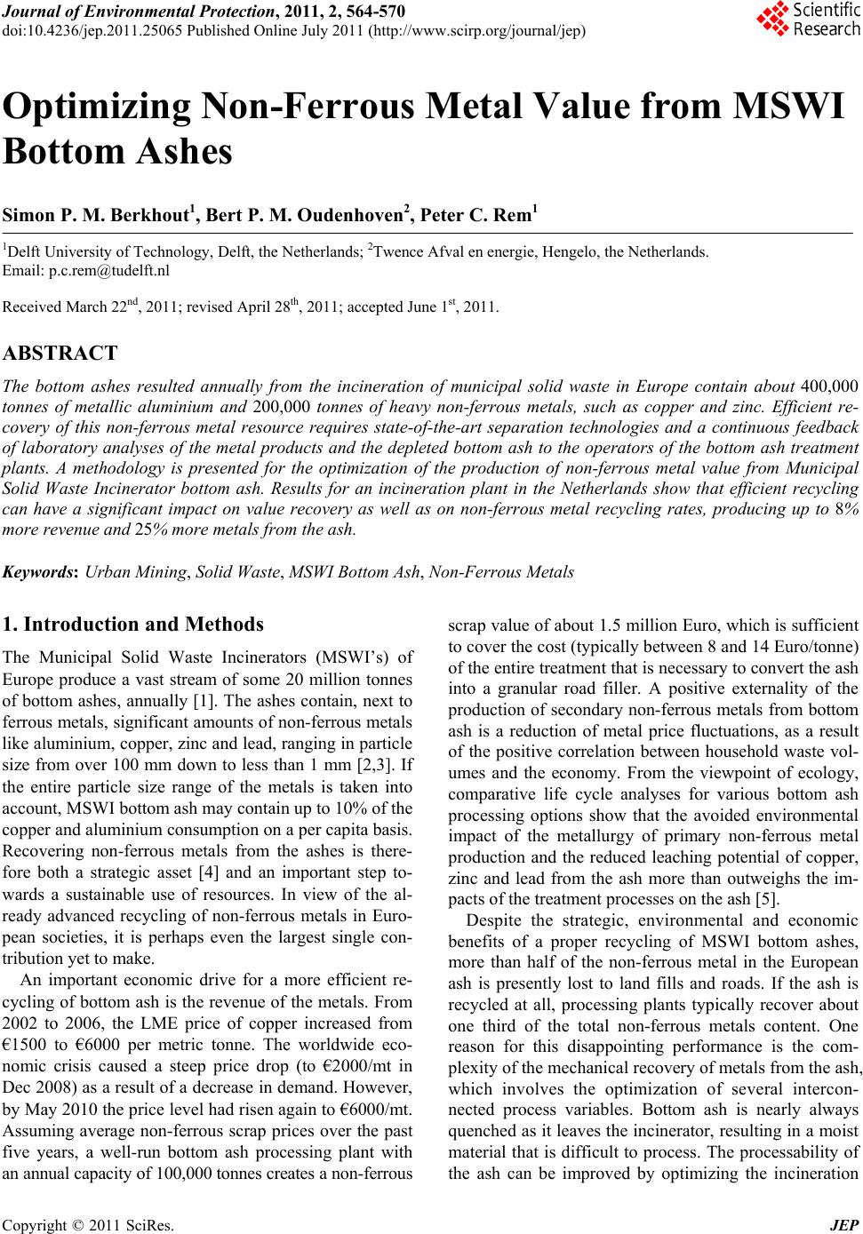
After removal of the magnetic particles, size fractions
larger than 2 mm were washed with water (L/S about 1)
in a rotating vessel for 15 minutes and the fines were
screened off. Then, the three alloy groups were separated
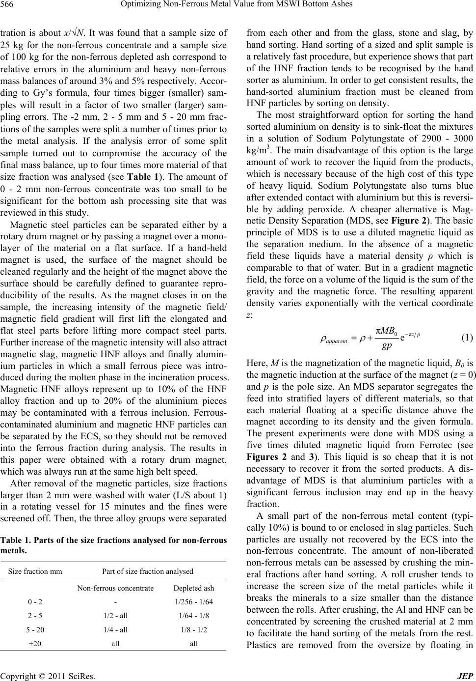
Table 1. Parts of the size fractions analysed for non-ferrous
metals.
Size fraction mm Part of size fraction analysed
Non-ferrous concentrate Depleted ash
0 - 2 - 1/256 - 1/64
2 - 5 1/2 - all 1/64 - 1/8
5 - 20 1/4 - all 1/8 - 1/2
+20 all all
from each other and from the glass, stone and slag, by
hand sorting. Hand sorting of a sized and split sample is
a relatively fast procedure, but experience shows that part
of the HNF fraction tends to be recognised by the hand
sorter as aluminium. In order to get consistent results, the
hand-sorted aluminium fraction must be cleaned from
HNF particles by sorting on density.
The most straightforward option for sorting the hand
sorted aluminium on density is to sink-float the mixtures
in a solution of Sodium Polytungstate of 2900 - 3000
kg/m3. The main disadvantage of this option is the large
amount of work to recover the liquid from the products,
which is necessary because of the high cost of this type
of heavy liquid. Sodium Polytungstate also turns blue
after extended contact with aluminium but this is reversi-
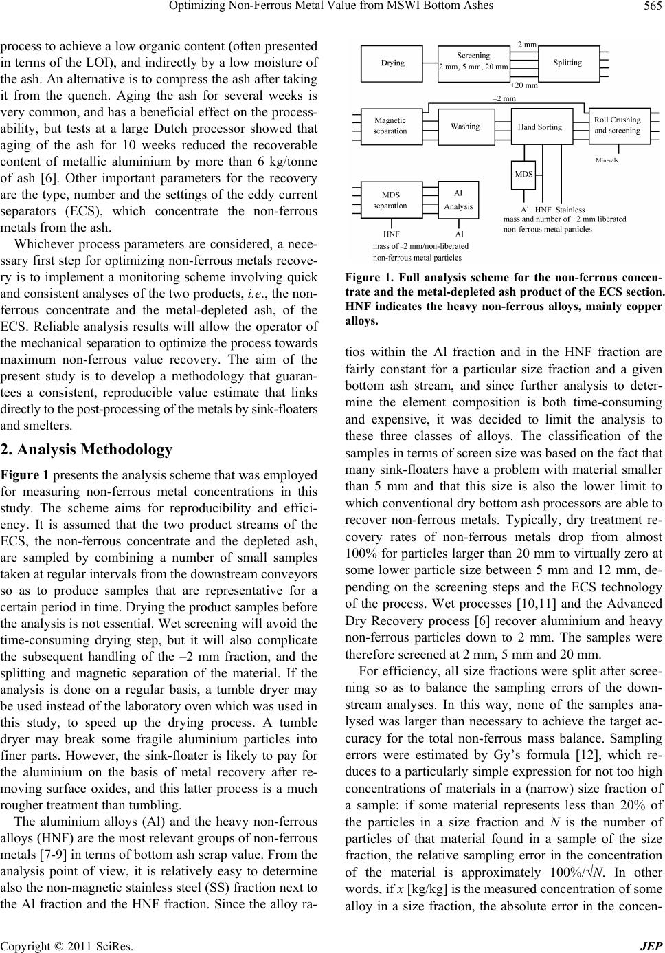
ble by adding peroxide. A cheaper alternative is Mag-
netic Density Separation (MDS, see Figure 2). The basic
principle of MDS is to use a diluted magnetic liquid as
the separation medium. In the absence of a magnetic
field these liquids have a material density ρ which is
comparable to that of water. But in a gradient magnetic
field, the force on a volume of the liquid is the sum of the
gravity and the magnetic force. The resulting apparent
density varies exponentially with the vertical coordinate
z:
π 0
πe
z
p
apparent
MB
gp


 (1)
Here, M is the magnetization of the magnetic liquid, B0 is
the magnetic induction at the surface of the magnet (z = 0)
and p is the pole size. An MDS separator segregates the
feed into stratified layers of different materials, so that
each material floating at a specific distance above the
magnet according to its density and the given formula.
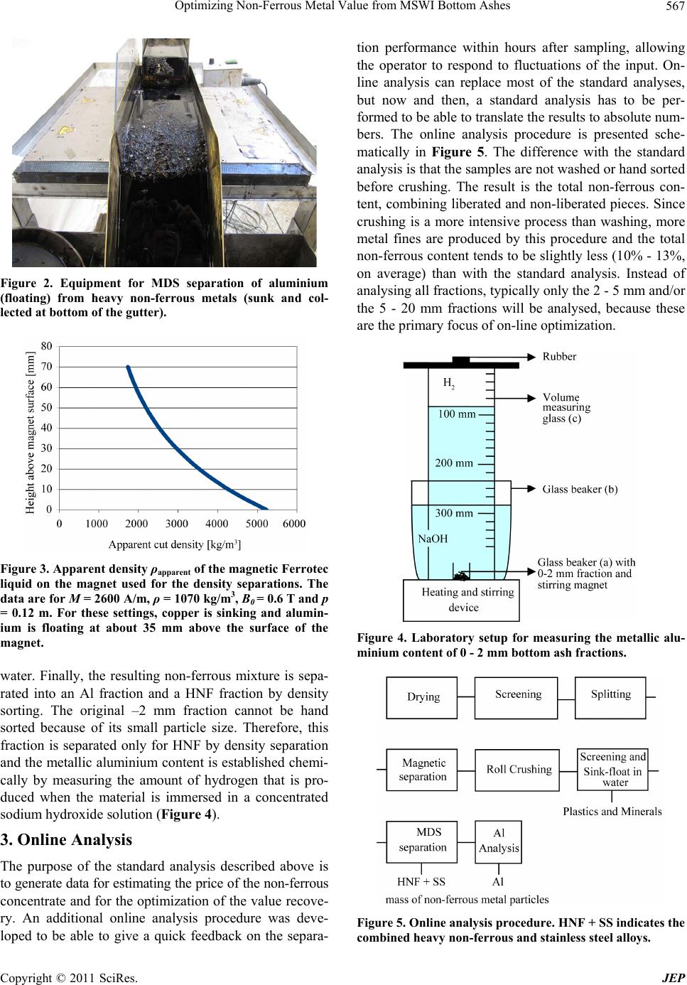
The present experiments were done with MDS using a
five times diluted magnetic liquid from Ferrotec (see
Figures 2 and 3). This liquid is so cheap that it is not
necessary to recover it from the sorted products. A dis-
advantage of MDS is that aluminium particles with a
significant ferrous inclusion may end up in the heavy
fraction.
A small part of the non-ferrous metal content (typi-
cally 10%) is bound to or enclosed in slag particles. Such
particles are usually not recovered by the ECS into the
non-ferrous concentrate. The amount of non-liberated
non-ferrous metals can be assessed by crushing the min-
eral fractions after hand sorting. A roll crusher tends to
increase the screen size of the metal particles while it
breaks the minerals to a size smaller than the distance
between the rolls. After crushing, the Al and HNF can be
concentrated by screening the crushed material at 2 mm
to facilitate the hand sorting of the metals from the rest.
Plastics are removed from the oversize by floating in
C opyright © 2011 SciRes. JEP

Optimizing Non-Ferrous Metal Value from MSWI Bottom Ashes567
Figure 2. Equipment for MDS separation of aluminium
(floating) from heavy non-ferrous metals (sunk and col-
lected at bottom of the gutter).
Figure 3. Apparent de nsity ρapparent of the magnetic Ferrotec
liquid on the magnet used for the density separations. The
data are for M = 2600 A/m, ρ = 1070 kg/m3, B0 = 0.6 T and p
= 0.12 m. For these settings, copper is sinking and alumin-
ium is floating at about 35 mm above the surface of the
magnet.
water. Finally, the resulting non-ferrous mixture is sepa-
rated into an Al fraction and a HNF fraction by density
sorting. The original –2 mm fraction cannot be hand
sorted because of its small particle size. Therefore, this
fraction is separated only for HNF by density separation
and the metallic aluminium content is established chemi-
cally by measuring the amount of hydrogen that is pro-
duced when the material is immersed in a concentrated
sodium hydroxide solution (Figure 4).
3. Online Analysis
The purpose of the standard analysis described above is
to generate data for estimating the price of the non-ferrous
concentrate and for the optimization of the value recove-
ry. An additional online analysis procedure was deve-
loped to be able to give a quick feedback on the separa-
tion performance within hours after sampling, allowing
the operator to respond to fluctuations of the input. On-
line analysis can replace most of the standard analyses,
but now and then, a standard analysis has to be per-
formed to be able to translate the results to absolute num-
bers. The online analysis procedure is presented sche-
matically in Figure 5. The difference with the standard
analysis is that the samples are not washed or hand sorted
before crushing. The result is the total non-ferrous con-
tent, combining liberated and non-liberated pieces. Since
crushing is a more intensive process than washing, more
metal fines are produced by this procedure and the total
non-ferrous content tends to be slightly less (10% - 13%,
on average) than with the standard analysis. Instead of
analysing all fractions, typically only the 2 - 5 mm and/or
the 5 - 20 mm fractions will be analysed, because these
are the primary focus of on-line optimization.
Figure 4. Laboratory setup for measuring the metallic alu-
minium content of 0 - 2 mm bottom ash fractions.
Figure 5. Online analysis procedure. HNF + SS indicates the
combined heavy non-ferrous and stainless steel alloys.

Optimizing Non-Ferrous Metal Value from MSWI Bottom Ashes 568
4. Results and Discussion
Table 2 shows results of a standard analysis for a sample
of the metal-depleted ash for a conventional dry treat-
ment process in the Netherlands. Next to the concentra-
tions of Al, HNF and SS, also the error estimates com-
puted by Gy’s formula are shown, to highlight the bal-
ance of contributions to the error in the overall non-ferrous
metal concentrations by the individual size fractions.
The data of Figure 6 represent averages of six analy-
ses performed over a three-month period. It is clear that
the recovery of aluminium and heavy non-ferrous alloys
drops to zero halfway the 5 - 20 mm fraction, which is
typical for conventional dry processes. Most ECS can
recover flat stainless steel particles starting from about
20 mm, and this is confirmed by the data. The overall
recoveries are about 50% for aluminium and 36% for the
heavy non-ferrous alloys. Figure 7 shows the effect of
the cut-point of the ECS in the grade-recovery curve for
aluminium. By changing the splitter position or the belt
speed of the ECS, the recovery of aluminium into the
non-ferrous concentrate can be increased at the expense
of recovering relatively more slag (mineral). The data
points show that although these settings are not the only
factor determining the aluminium recovery, they are
nevertheless a major one. The line drawn through the
data was made by connecting the point of zero recovery
and 100% aluminium grade with the point of 100% re-
covery of the ECS input and the input aluminium grade.
These two extreme points can be realised by moving the
splitter of the ECS so as to recover either all or none of
the input material into the non-ferrous concentrate.
To optimize value recovery, an estimator is needed for
the price of the non-ferrous concentrate. Sink-floaters
will typically offer prices for MSWI non-ferrous scrap
based on formulas that include the costs of sink-floating,
smelting and the LME prices for the pure metals. A sim-
ple formula for the revenue of scrap in Euro/tonne is
given by Equation (2):



S
AlAl AlCuCu
SF
S
Al
Al
Cu
Revenue(100%F )
RLMEF Al%LMEFCu%
L Slag%F
F Sales fee
R Recovery of aluminium from the smelt
F Aluminum smelter fee
F Copper smelter fee
L



SF
Al
Cu
Land fill fee
F Sink-float fee
LME LME price of Aluminium
LME LME price of Copper
(2)
Figure 6. Average ECS input metal contents and recoveries
of aluminium (Al, top), heavy non-ferrous (HNF, middle)
and stainless steel (SS, bottom) for a Dutch conventional
dry process in terms of kg per tonne of dry ECS input. The
results have been averaged over six analyses performed in a
period of three months.
Figure 7. Grade-recovery curve for aluminium in the non-
ferrous concentrate stream.
C opyright © 2011 SciRes. JEP

Optimizing Non-Ferrous Metal Value from MSWI Bottom Ashes 569
Table 2. Example result for the analysis of a sample from the metal-depleted product stream, including the number of parti-
cles (#) found in each split fr ac tion.
Size fraction Aluminium Heavy non-ferrousStainless
mm kg
Spl.
kg # kg # kg #
Aluminium
%
Heavy non-ferrous
%
Stainless
%
0 - 2 47.8 256 0.0012 0.00082 0 0.26 0.18 0.0
2 - 5 15.8 8 0.0446 1850 0.0307 3440 0 0.31 ± 0.010.22 ± 0.01 0.0
5 - 20 37.8 2 0.2750 1041 0.188 1710.014110.48 ± 0.010.33 ± 0.03 0.02 ± 0.01
+20 12.8 1 0.0426 19 0.0123 13 0.0564110.04 ± 0.010.01 ± 0,00 0.05 ± 0.01
Total 114.2 1.09 ± 0.020.74 ± 0.03 0.07 ± 0.02
Figure 8 shows a comparison of the prediction of this
formula against historic scrap revenues for a Dutch
MSWI over a five-year period, assuming a sales fee of
10%, a recovery of aluminium from the smelt of 70%,
smelter fees of 300 Euro/tonne for aluminium and 900
Euro/tonne for copper and a sink-float fee of 90 Euro/
tonne. The land fill fee was set to 0 Euro/tonne, be-
causein this case the slag separated by the sink-floater
was returned to the MSWI. During the five-year refer-
ence period, the primary data for the non-ferrous concen-
trate showed a variation in slag content from 10% to 55%,
and the LME prices for copper and aluminium varied by
a factor of 2. Despite such variations, Equation (2) gives
a reasonable account of the fluctuations of the actual
non-ferrous scrap revenues obtained by the MSWI. There-
fore it is realistic to use such equations in optimization
studies, provided that the non-ferrous grade of concen-
trates remains within the limits of the validation data.
Figure 9 shows the results of the recovery-recovery
graph for aluminium and copper versus slag in the
non-ferrous concentrate computed from seven experi-
mental data points. The trend line shows a positive cor-
relation between both recoveries. This is expected be-
cause changes of the cut-point of the ECS to recover
more non-ferrous metals will also increase the amount of
slag in the non-ferrous product. However, it is remark-
able that 25% more non-ferrous metal can be recovered
per tonne of input bottom ash by allowing the slag con-
tent of the non-ferrous product to increase from 25% to
58%. Figure 10 shows a translation of the recovery trend
lines into a curve for the revenue per tonne of dry ECS
input. The LME prices used in Equation 2 are 1600
Euro/tonne for aluminium and 4,400 Euro/tonne for
copper, in correspondence with 2010 trend line figures
for these metal prices. The curve indicates that within the
range of slag contents covered by the validation data,
revenues per tonne of input bottom ash increase with the
volume of non-ferrous product (and so with slag content).
This means that in order to optimize value recovery, the
ECS operator should go for high non-ferrous recovery
Figure 8. Comparison of actual scrap prices with the pre-
dictions of Equation (2).
Figure 9. Recovery of non-ferrous metals versus recovery of
slag into the non-ferrous product of the ECS.
Figure 10. Revenue of the non-ferrous product, per tonne of
bottom ash input to the ECS.

Optimizing Non-Ferrous Metal Value from MSWI Bottom Ashes 570
and not for high non-ferrous grade. Such a strategy is
counterintuitive to most operators but it will increase
revenues by up to 8% and is also beneficial for the recy-
cling rate of non-ferrous metals from waste. In this as-
pect, the result of this study is remarkably parallel to that
of a study to optimize non-ferrous value recovery from
car scrap, more than a decade ago [13]. That study also
concluded that ECS operators may gain 25% extra non-
ferrous metals by going for recovery instead of grade,
increasing non-ferrous metal revenue by 15%.
REFERENCES
[1] EU Statistics, “Structural Indicators: Municipal Waste,”
2007. http://Europe.eu.int.
[2] L. Muchova and P. C. Rem, “Hydrogen from Bottom
Ash,” In: A. Kungolos, K. Aravossis, A. Karagiannidis
and P. Samaras, Eds., Proceedings of the International
Conference on Environmental Management Engineering,
Planning, GRAFIMA, Thessaloniki, 2007, pp. 1895-
1900.
[3] Y. Hu and M. C. Bakker, “Recovery and Distribution of
Incinerated Aluminium Packaging Waste,” Submitted to
Waste Management, 2010.
[4] Public Consultation of the European Union, 2006.
[5] L. Muchova, “Wet Physical Separation of MSWI Bottom
Ash,” TU Delft PhD Thesis, 2010.
[6] W. de Vries, P. Rem and P. Berkhout, “ADR: A New
Method for Dry Classification,” Proceedings of the ISWA
International Conference, Lisbon, 12-15 October 2009, p.
103.
[7] J. M. Chimenos, M. Segarra, M. A. Fernandez and F.
Espiell, “Characterization of the Bottom Ash in Munici-
pal Solid Waste Incinerator,” Journal of Hazardous Ma-
terials, Vol. 64, No. 3, 1999, pp. 211-222.
doi:10.1016/S0304-3894(98)00246-5
[8] G. Schmelzer, S. Wolf and H. Hoberg, “New Wet Treat-
ment for Components of Incineration Slag,” Aufbercei-
tungs-Technik, Vol. 37, No. 4, 1996, pp. 149-157.
[9] L. Muchova, E. J. Bakker and P. C. Rem, “Precious Met-
als in Municipal Solid Waste Incineration Bottom Ash,”
Water Air Soil Pollution, Vol. 9, No. 1-2, 2009, pp. 107-
116. doi:10.1007/s11267-008-9191-9
[10] P. C. Rem, C. de Vries, L. A. van Kooy and P. Bevilac-
qua, M. A. Reuter, “The Amsterdam Pilot on Bottom
Ash,” Minerals Engineering, Vol. 17, No. 2, 2004, pp.
363-365. doi:10.1016/j.mineng.2003.11.009
[11] BREF Waste Incineration, “Integrated Pollution Preven-
tion and Control: Reference document on the Best Avail-
able Techniques for Waste Incineration,” July 2005.
[12] P. Gy, “Sampling for Analytical Purposes,” ISBN
0471979562, John Wiley, Hoboken, 1998.
[13] A. J. Gesing, D. Reno, R. Grisier, R. Dalton and R. Wo-
lanski, “Nonferrous Metal Recovery from Auto Shredder
Residue Using Eddy Current Separators,” In: B. Mishra,
Ed., Proceedings of the EPD Congress, 1998, TMS (1998)
9.
C opyright © 2011 SciRes. JEP