Engineering, 2011, 3, 669-679
doi:10.4236/eng.2011.37080 Published Online July 2011 (http://www.SciRP.org/journal/eng)
Equivalence Theory Applied to Anisotropic Thin Plates
Madjid Haddad, Yves Gourinat, Miguel Charlotte
Université de Toulouse, INSA, UPS, Mines d’Albi, ISAE, Institut Clément ADER (ICA), Toulouse, France
Received October 18, 2010; revised June 10, 2011; accepte d J u ne 20, 2011
Abstract
We extend the Equivalence Theory (ET) formulated by Absi [1] for the statics of isotropic materials to the
statics and dynamics of orthotropic materials. That theory relies on the assumption that any real body mod-
eling may be substituted by another one that, even though it may possibly have material constitutive laws
and geomet- ric properties with no physical sense (like negative cross sections or Young modulus), is in-
tended to be more advantageous for calculus. In our approach, the equivalence is expressed by equating both
the effective strain energies of the two models and the material structural weights in dynamics [2]. We pro-
vide a numerical analysis of the convergence properties of ET approach while comparing its numerical re-
sults with those pre- dicted by the analytical theory and the Finite Elements Method for thin plates.
Keywords: Equivalence Theory, Thin Plates, Anisotropic Plates, Dynamics
1. Introduction
Around the 70s some researchers [1,3] were interested in
the problem of modelling a slab as a beam lattice or truss.
Such a substitution relies on some common engineering
viewpoint according which if the slab can be subdivided
into slices parallel to its boundaries (like AB or CD on
Figures 1 and 2), then each slice may be assimilated to a
beam with related material and geometrical properties.
This coarse structure approach which is suitable for
pre-sizing was also assumed to be applicable to the cal-
culation of arch dams (Figure 3) sliced into arcs (AB)
and consoles (CD).
Such a practical problem gave birth to the Equivalence
Theory (ET) developed by Absi [1] who specified the
general conditions of equivalence in statics for isotropic
materials. In statics, the standard equivalence criterion is
expressed between the strain energies. That theory as-
sumes that any real body modelling may be substituted
by another one that, even though it may possibly have
material constitutive laws and geometric properties with
no physical meanings (like negative cross sections or
Young modulus), is intended to be more advantageous
for calculus. In the literature [1,2,4], only few investiga-
tions have tried to check this assumption. These equiva-
lence analyses were formulated for the statics of different
cases of isotropic slabs and the comparisons made with
the analytical theory and the Finite Element Method
(FEM) analysis have led to very encouraging conclusions.
However, the ET has been abandoned in favour of the
FEM because the latter is more flexible to deal with
structures with arbitrary geometry.
Figure 1. Rectangular slab subdivided into slices parallel to
its boundaries.
Figure 2. Lozenge slab subdivided into slices parallel to its
boundaries.
Figure 3. Arch dam subdivided into arcs.

M. HADDAD ET AL.
670
This work aims to extend the ET approach to the
analysis of anisotropic plates subjected to transverse
loads, in statics, and to study the frequencies and the
modes shapes in dynamics. To check the validity of the
extended formulation, numerical comparisons with ana-
lytical solutions in statics and to FEM results in dynam-
ics are made. As mentioned previously, the possible lack
of meaning of the resulting equivalent model makes the
treatment of such a method on commercial FEM soft-
ware (Patran/Nastran, Catia...) difficult, if not impossible.
Therefore in order to compare our new improvement of
the theory and overcome these difficulties, we were led
to develop a finite element computer codes in Matlab.
2. Formulation of the Method in Statics
The Equivalence Theory (ET) aims at replacing a given
real body by another arbitrary chosen, and possibly ficti-
tious, one [1]. The standard equivalence criterion is ex-
pressed between the strain energies. Here we will choose
the substituting body as a lattice structure with beams
elements. We will first express the energy of tensile and
bending of an anisotropic plate. Then, according with the
ET, we will identify the cross sections, the quadratic
moments and the central moments of inertia of beams, by
making a comparison between the Elementary Repre-
sentative Cells (ERC) of the two models.
2.1. Expressing Equivalence in Traction
2.1.1. Ela sti c E n erg y of an Orthotropi c Plate: [4]
Consider the case of a thin, linearly elastic and anisot-
ropic plate, with three planes of symmetry and a constant
thickness h. The plate stress strain relations are written in
this case as follows:
;
;2
xxx y
y
yyx xyxy
EE
EE G


 
  
   (1)
with
x
l
EkE
; yt
EkE
; tl llt t
EkEkE




; lt GG

Hereabove ,,
x
yxy

 denote respectively the normal
stresses with respect to x and y axes, and the shear stress,
while
1
;;
2
xyxy
uv uv
x
xxy


 
 

 

(2)
are respectively the related normal and shear strains;
besides El and Et: are respectively the longitudinal and
transversal Young’s moduli, lt

and t
tllt l
E
E
  are
the longitudinal and transversal Poisson’s ratios, which
provide

1
1lt tl
k


, and Glt is the Coulomb’s coeffi-
cient.
Suppose now that the plate is subjected to a uniform
bi-axial tensile along the x and y axis. Hence its elastic
energy reads like

22 2
22
2
p
txxyyxyxy
A
UEEE G
 
 
 (3)
where Ap represents the ERC surface area of the plate
while noticing that the strains are independent on x, y or
z. Note that we recover the traction energy of a mate-
rially isotropic plates in plane stress for tl
EE E


(the same Young’s modulus) and tl lt

  (same
Poisson’s ratio).
2.1.2. Beam Traction Energy
The traction energie of a beam “ij”, Figure 4 is:
2
22
11 2212
cossin2sin cos
ij ij
We ee






 (4)
where ijij e
ES l


is a characteristic traction parameter,
while Sij, le and E are respectively the cross section,
length and Young’s modulus of the beam.
2.1.3. Expressing the Traction Equivalence
The equivalence is expressed in an elementary represen-
tative cell ERC of the two structures.
Consider the cell represented in Figure 5.
The strain energy expressions of the different beams
constituting this cell are:


2
11
2
22
2
22
11 2212
2
22
11 2212
1
2
1
2
1cossin2sin cos
2
1cossin2sin cos
2
AB CDAB
AC BDAC
AD AD
BC BD
WW e
WW e
Weee
Weee






 
 

 



 


(5)
Figure 4. A beam representation in the plane.
Figure 5. ERC “square with diagonals”.

M. HADDAD ET AL.
671
Write the equivalence between the two cells, we have
then:
 
 
22 2
112211 2212
22
11 22
2
22
11 2212
2
22
11 2212
22
2
1cossin2sin cos
2
1cossin2sin cos
2
p
t
AB AC
AD
BD
A
UEeEeEeeGea
xy
ee
ee e
eee

 


  









(6)
Taking ADBD

, and comparing the two terms of
the Equation (6) we can write:

222
4
1111 11
4
cos
2
cos
2
px AB AD
px
AB AD
AE eee
AE






(7)
 
222
4
2222 22
4
sin
2
sin
2
py AC AD
py
AC AD
AE eee
AE






(8)
 
22
22
12 12
22
4sincos
1
4sin cos
pAD
p
AD
A
Ge e
AG



 (9)

22
11 2211 22
22
2sincos
1
2sin cos
pAD
p
AD
A
Eee ee
AE


 

 (10)
Replacing AD

in the Equations (7) and (8), we ob-
tain:

2
1cot
2
pl
AB tl
AE
k

  (11)

2
1tan
2
pt
AC lt
AE
k

  (12)
22
2sin cos
pl tl
AD
AE




 (13)
We know that:

AB AB
EA a  ,

AC AC
EA b   and

AD AD
EA l  ;
where Aij, Eij are respectively the cross section and the
Young’s modulus of the beam “ij” and a, b, l: lengths of
the considered beam, as shown in Figure 5.
Let’s consider that the beams which are parallel to the
x axis and the diagonal ones have the same Young’s
modulus as the longitudinal one of the plate, and those
which are parallel to the y axis, have the same Young’s
modulus as the transverse one of the plate.
Finally, we obtain:

2
1cot
2
AB lt
bh
Ak

  ;

2
1tan
2
AC lt
ah
Ak

  ;
22
2sin cos
lt
AD abh
Ak
l






.
2.2. Bending Equivalence
2.2.1. Plate Bending Energy
In our study we consider the Kirchoff-Love’s plates,
which suppose that the straight linear elements that are
perpendicular to the plate’s mean surface still remain so
even after deformation.
We have:
22 2
22
;; .
xyxy
ww w
zz z
x
y xy

 
 
 (14)
Then the bending and tensional moments are given as
follows:
/2 22
1
22
/2
/2 22
1
22
/2
/2 2
/2
d
d
d2
h
xx x
h
h
yy y
h
h
xy xyxy
h
ww
MzzDD
x
y
ww
MzzDD
yx
w
MzzD
xy
























(15)
where
3
12
x
x
Eh
D

;
3
12
y
y
Eh
D

;
3
112
Eh
D ;
3
12
xy Gh
D.
The bending energy of the plate is given [5]:
22
1
ddd
2xy xy
ww w
VMM Mxy
xy
xy

 
  
 
 



 


,
(16)
which gives:
2
2
22
2
122
1
d2
2dd
xy
ww
VD D
xy
xy
ww w
DDxy
xy xy








 


 
 



  
  
(17)
with:
3
12
l
x
kE h
D;
3
12
t
y
kE h
D;
3
112
tl l
kEh
D

;
3
12
lt
xy
Gh
D.

M. HADDAD ET AL.
672
2.2.2. Bending and Torsional Energie of a Beam
The bending and tensional energy contributions of a
beam ‘ij’(see [1,5]) are respectively given as
22
22
22
2
2
1cos sin
2
cossin
fij
ww
Wxy
w
xy




 





 
(18)
where

ije ij
EIl 
 is defined with the quadratic mo-
ment I of the cross section Sij and
2
22 2
22
11 sin 2cos 2
22
tww w
Wxy
yx





 


 






 (19)
where e GJl


.
2.2.3. Expressing the Bending Equivalence
Here we will assume that all the beams work in bending
and only the longitudinal and diagonal ones work in tor-
sion (Figure 6). This supposition has no effect in the
theory itself, since the unique condition to satisfy is to
conserve the total strain energy. We can write then:
22
22
2
11
22
fAB fCDABAB
ww
WW
x
y x




 

 

22
22
2
11
22
fAC fBSACAC
ww
WW
x
y y

 

  
 


 
2
222
22
22
1cossincos sin
2
fADAD www
Wxy
xy




 




2
222
22
222
1cossincossin
2
fBCBC www
Wxyxy









The equivalence is given by equating the two strain energies:
2222
f
AB fBCfAC fADtABtAC
WSV WWWWWW   (20)
22
22
222
1
22222 2
2
22 222 2
22 22
22 22
2'
2
11
cossin2sin coscossin2
22
x yxyABAC
AD BD
Sww wwwww
DDD D
xy
xyxyx y
ww www
xy
xy xy



   
 
 

 
   
 

 
   


  

 


 

2
22
22
sin cos
AB AC
w
xy
ww
xy xy














 

(21)
Let now AD BD



 we can write:
222
222
4
222
4
cos
2
cos
2
xAB AD
x
AB AD
SD www
xxx
SD



 



 

 
 
(22)
222
222
4
222
4
sin
2
sin
2
yAC AD
y
AC AD
SD www
yyy
SD



 



 

 


(23)
22 22
22
122 22
1
22
2sincos
1
2sin cos
AD
AD
ww ww
SD
x
yxy
SD


 


 

(24)
22
22
22
22
22
22
24sincos
24sincos
xy AD
AB AC
AB ACxyAD
ww
SD xy xy
ww
x
yxy
SD


 





 





 


 
(25)
Replace the value of AD


in the different equations,
we have then:
2
1cot
22
x
AB
SD SD


;
2
1tan
22
y
AC
SD SD


 ;
1
22
1
2sin cos
ADCB SD




 ;

M. HADDAD ET AL.
673
Figure 6. ERC «square with diagonals».


1
2
AB ACxy
SD D   
We know that: ABl AB EI a

, ACt AC
EIb

,
ADl AD
EI l

, ABlt AB
GJ a

 and AClt AC GJ b


Here Iij and Jij denote respectively the second and po-
lar moments of the cross section area of the beam “ij”.
By substituting these values in (36), it comes then:

3
2
1cot
24
AB tl
bh
Ik

  ;

3
2
1tan
24
AC lt
ah
Ik

  ;
3
22
24 sin cos
tl
AD abh
Ik
l






;

3
1
6
tl l
AB AClt
E
abh
JJ k
ab G


 


.
3. Static Validation
3.1. Simply Supported Plate Submitted to
Uniform Distributed Load (Figure 7)
Consider that the plate has the following geometrical and
material properties: length L = 1 m; width l = 0.8 m, and
thickness h = 1 mm, longitudinal and transversal
Young’s moduli: El = 11.109 Pa and Et = 11.106 Pa,
Poisson’s ratio: 0.3
lt

, Coulomb’s coefficient: Glt =
40.106 Pa. That plate is submitted to a uniform constant
load q0 = 1 Pa.
The theoretical transverse displacement solution of
this orthotropic plate problem at any given point with
coordinates (x, y) is given in [6] page 59 as

11
ππ
,sinsin
mn
nm
mx ny
wxyW Ll





 (26)
with

4
4222 44
1112 6622
4
π22
mn
mn
q
W
DmDD mnrDnr
a


 



(27)
Figure 7. Simply supported plate submitted to uniform
distributed load.
rLl

and
0
2
16 for, 1,3,5,
π
mn
q
qmn
mn

 (28).
The deformed shape obtained after loading is given in
Figure 8.
A comparison between the theoretical deformation and
the one given by the ET, along the two median lines, X =
0.5 and Y = 0.4, is shown in Figure 9.
To evaluate the accuracy of this method, a comparison
with the FEM software Patran/Nastran is done for the
same size of the mesh and number of nodes as in ET.
Quadratic elements are chosen to mesh the thin plate
structure in Patran/Nastran. The different results are re-
sumed in Table 1, and compared to the theoretical dis-
placement in the plate center wtheoric = 0.0142368 m.
While a better accuracy is reached with the FEM method,
as expected, very good agreements are observed between
the FEM and ET and even the accuracy with the later
still remains good for relatively coarse mesh sizes.
Moreover, the convergence to the theoretical solution is
also observed with increasing the mesh density.
3.2. Simply Supported Plate Submitted to
Concentrated Load Applied in Its Center
Let us consider the previous thin plate is now loaded at
its center by a concentrated force of magnitude P = 0.01
N.
The theoretical expression of the displacement solu-
tion given in (26) and (27) stay the same, except that
00
4sin πsin π
mn
x
y
P
qmn
Ll Ll



(29)
The deformation caused by this load is represented in
Figure 10. The related deformation obtained by the ET
approach is represented on Figure 11 and a comparison
with the theoretical solution is performed along the two
median lines in Figure 11.
The Table 2 provides the related numerical values
with in addition the results obtained by the FEM theory
obtained for the same size mesh, (same number of nodes).
The calculation of the theoretical displacement in the

M. HADDAD ET AL.
674
Figure 8. Deformation under a uniform distribute d load.
(a)
(b)
Figure 9. (a) Superposition of the median lines displace-
ments along the “X” axis; (b) Superposition of the median
lines displacements along the “Y” axis.
Table 1. Comparison of the central deformation for a sim-
ply supported plate under a unifor m loading.
mesh
size
FEM
deformation
[m]
EM
deformation
[m]
Error
FEM (%)
Error ET
(%)
10 × 8 1.405E-02 1.340E-02 –1.34% –4.59%
20 × 16 1.422E-02 1.378E-02 –0.12% –3.11%
30 × 24 1.425E-02 1.390E-02 0.08% –2.46%
plate center gave wtheoric = 0.00132144758109 m. Once
again, we observe that the two methods converge to the
theoretical solution, when we increase the mesh size.
Unlike the first example, we observe here (as the main
result of the statics section) that the ET provides better
results than those of the FEM.
4. Application of the Equivalence Theory in
Dynamics
In statics we have observed that the ET provides very
good results, which are in agreement with the literature
[1-3], and we have obtained the same conclusions with
anisotropic plates. Now we will test this method in dy-
namics.
In our study we consider the mass conservation of the
system. By equating the overall masses of the continuous
plate and lattice models, and supposing that a homoge-
neous mass density in the lattice structure, we have:
1
N
P
ee
e
LlhA a 


 
and so
1
P
N
ee
e
Llh
A
a







(30)
with ,
ee
A
a are respectively the cross section and length
of the eth beam, N is the number of the beams,

the
mass density of the beams,
p

the mass density of the
plate, L, l and h are respectively the length, width and
thickness of the plate.
To calculate the inertial moment of the beams we have
to precise a shape for the cross sections. We choose cir-
cular ones, having the section from the static equivalence;
we calculate first the beam cross section radii π
ee
RA
and their inertial moment
²
2
ee
e
lAR
I



 (31)
5. Example: Clumped Rectangular Plate
5.1. Frequencies
The plate considered here is the same as in the first ex-
ample, we have just clamped it in its four sides.
In dynamics we preferred to compare the ET results to
the FEM ones. We have choose a mesh of 200 × 160
elements in Nastran/Patran software, and we defined the
plate as a shell element, these was to approximate better
the real solutions.
In what follows we will show the first hundred “100”
frequency values obtained for different mesh sizes, and
for two representations of the mass matrix, the first is the
consistent mass matrix, which is the same expressed in
the classic “FEM” formulation, and the second one is the
lumped mass matrix, whish considered that the mass and

M. HADDAD ET AL.
675
Figure 10. Deformed shape under a before concentred cen-
tred load.
(a)
(b)
Figure 11. Superposition of the results among the median
lines (A-X = 0.5 ; B-Y = 0.4).
Table 2. Comparison of the central deformation for a sim-
ply supported plate under a c oncentrated load applied in its
center.
mesh
size
FEM
deformation
[m]
EM
deformation
[m]
Error FEM
(%)
Error ET
(%)
10 × 8 1.417E-03 1.291E-03 9.78% –2.34%
20 × 16 1.367E-03 1.321E-03 3.49% –0.02%
30 × 24 1.348E-03 1.325E-03 1.77% 0.24%
the inertial moment is equitably distributed in the nodes
of the beams. Moreover we will have for the translation
the half mass working in the three direction “u, v, w” and
the half inertial moment working in the three rotating
directions “,,
x
yz

 ” .Note that the bending isn’t con-
sidered here, this approach is the same as the
Patran/Nastran one for the lumped mass matrix.
Figure 12 shows the first hundred eigenvalues of the
plate obtained by the ET and confronts them with the
values obtained by finite element method. We see very
clearly that when the mesh size in the ET is increasing,
the curve obtained by this method tends to approximate
that obtained by FEM. We also note that even with a
coarse size mesh, the first eigenvalues are very close to
those obtained by the FEM. The evolution of the relative
discrepancy between the ET results versus the FEM ones
is plotted in Figure 13. In fact, we observe that the first
five “5” frequencies obtained are very close to those ob-
tained by FEM even when we use small size mesh. The
convergence as the number of elements is increasing is
very remarkable, we note that the first hundred “100”
frequencies are obtained with a maximum error of 25%
for a mesh of (20 × 16) to 12% for a mesh of (30 × 24).
The convergence is also observed in the case a distrib-
uted (lumped) mass matrix. Indeed we notice that with
the mesh size of (20 × 16) we have a maximum error of
86%, this error is reduced to 16% for a mesh size of (30
× 24). We clearly note that the best results are obtained
for a consistent weight distribution.
5.2. Mode Shapes
Figure 14 illustrates the first ten mode shapes obtained
by the ET approach. These mode shapes are exactly the
same than those found in literature [7].
6. Conclusions
Heretofore the equivalence theory has been expressed
only for isotropic static problems. The formulation is
based in equating the strain energies of two systems. The
researchers [1,3,4] were interested by the calculation of
deformations, bending moments, convergence with in-
creasing mesh size. They found that in statics this
method is very robust, it gives very good results with
small mesh sizes and the results are converging when we
increase the mesh size.
This method may provide a sheap, sufficient reliable,
and convient approach to treat complex structural sys-
tems as the computer storage requirement and running
times are small compared with those of other numerical
methods.
In order to demonstrate the validity of the procedure

M. HADDAD ET AL.
676
(a) (b)
Figure 12. Comparison of the first hundred frequencies obtained by the ET and those provided by the software Patran/
Nastran. (a) Lumped mass matrix; (b) Consistent mass matrix.

M. HADDAD ET AL.
677
(a) (b)
Figure 13. Errors obtained for the first hundred fre que nc ies. (a) Lumped mass matrix; (b) Consistent mass matrix.

M. HADDAD ET AL.
678
mode 1 mode 2
mode 3 mode 4
mode 5 mode 6
mode 7 mode 8
mode 9 mode 10
Figure 14. Mode shapes of orthotropic clumped plate.

M. HADDAD ET AL.
679
for anisotropic static problems, two example problems,
relevant to plane stress (thin plates) were examined by
using the ET approach and the FEM with different grid
arrangement. The results are in good agreement with the
analytical solutions even in the case of a small number of
nodes (coarse mesh). Most importantly, we have also
noted that these results are very near and even in some
cases better than those predicted by the FEM.
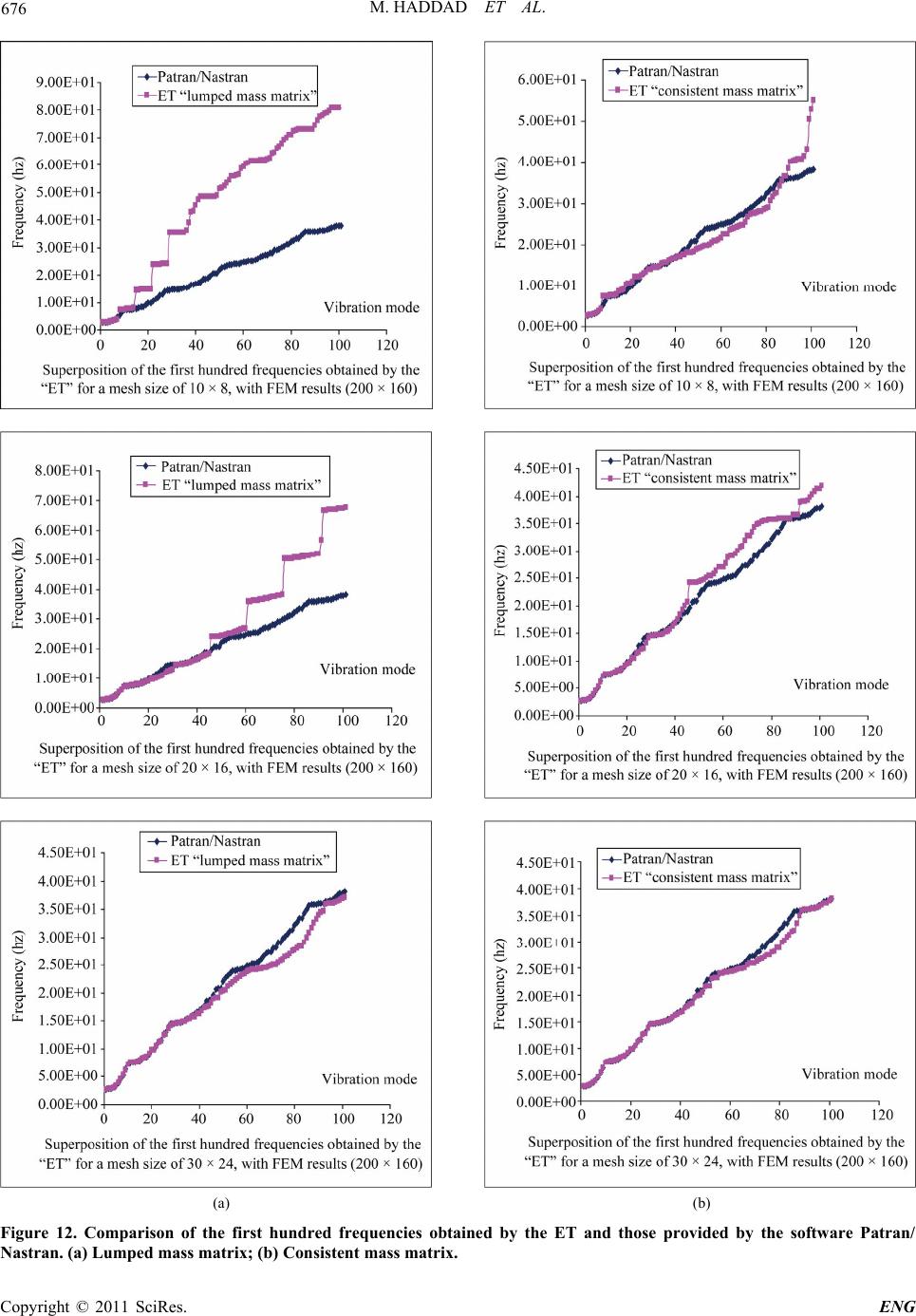
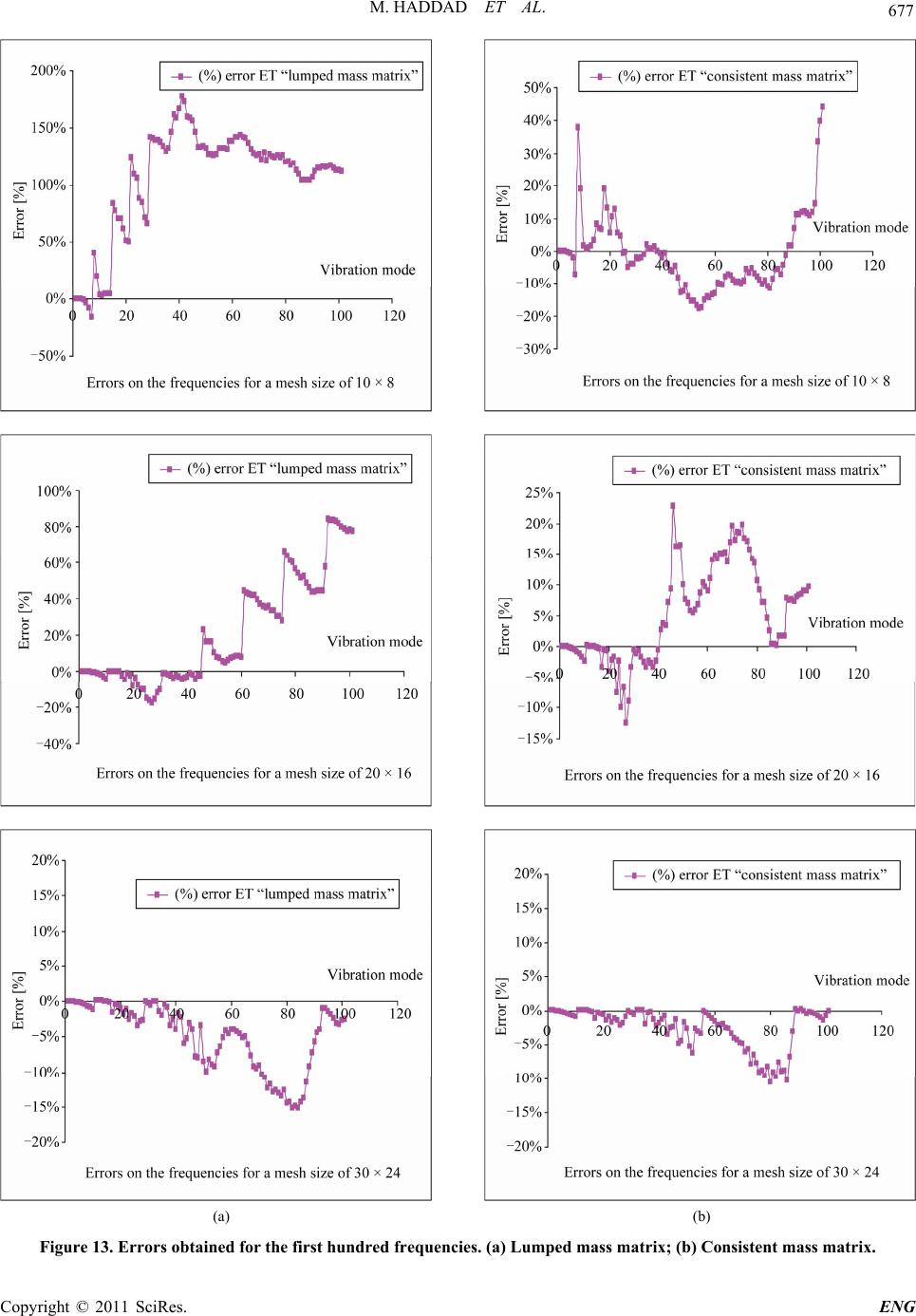
To extend this procedure to dynamics, we have just
formulated in addition a simple mass conservation rule,
and choose a circular form for our beams. In order to
validate this procedure, we compared the results to those
of the FEM with a relatively fine mesh. We have not
made a comparison with analytical solutions because this
latter proposes approximate solutions concerning only
the bending of the plates, while the FEM gives the dif-
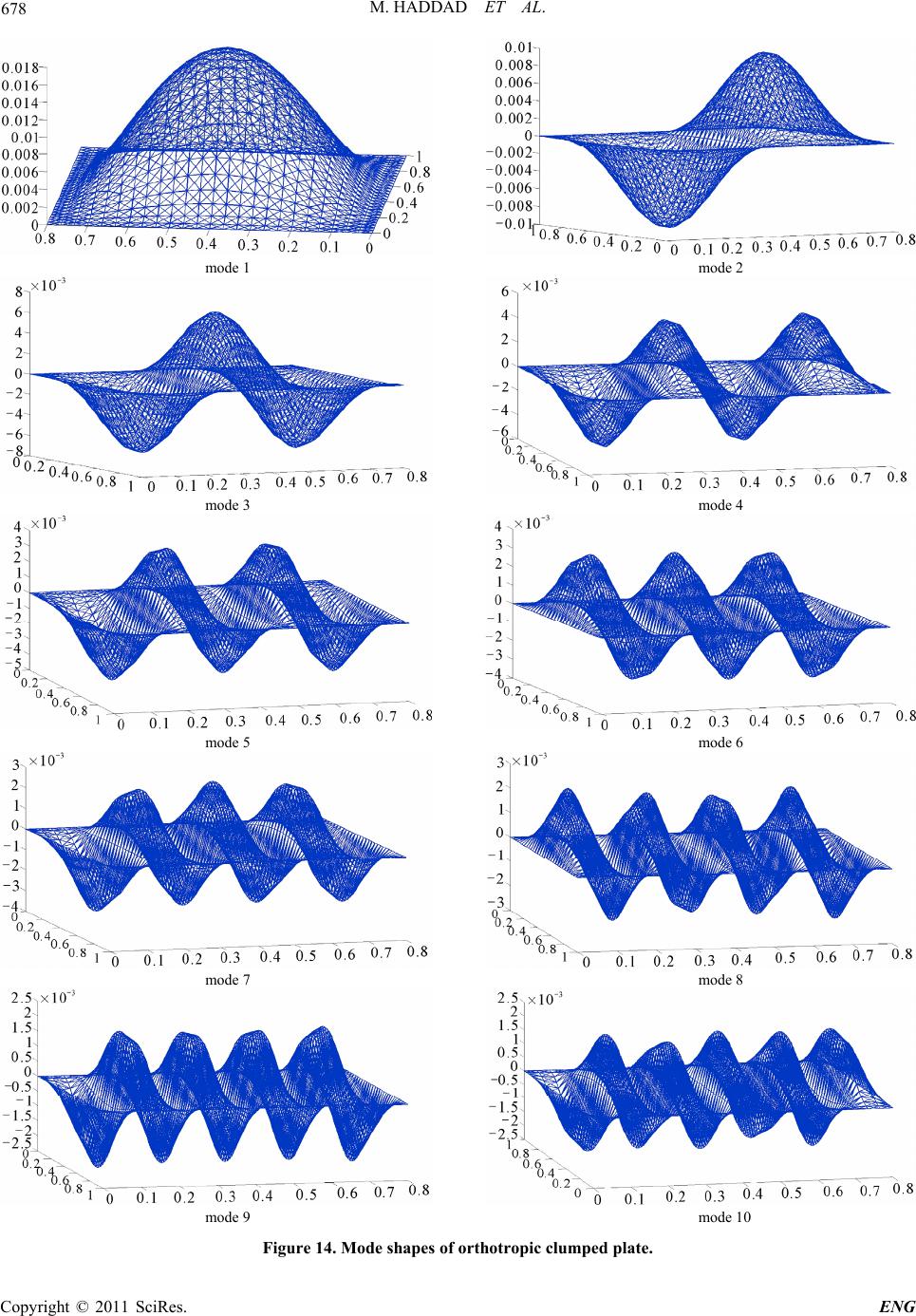
ferent vibration modes (bending, torsion, traction…). We
considered the problem of a thin clamped plate, and
found that the results are in good agreement with the
FEM solutions. We note also that the formulation of the
mass as a consistent one gave best results; this results are
explained by the fact that the mass is well distributed in
the ERC and approaches the homogeneous distribution in
the real cell. The lumped representation of the mass is
found to be convenient in the high computational speed,
indeed the mass matrixes are diagonals, and so easier to
invert, moreover we observe that its results remain close
to those of a consistent formulation. Thus the user can be
free to choose between very accurate results and high
computational speed.
A future work could be to deal with 3D problems. We
have created the connectivity table of different 3D
“ERC”, and begin the solving of the problem concerning
the expression of the stiffness matrix in 3D. The analysis
performed for the 2D models can be extended to the 3D
ones and also addresses other problems like fatigue and
blucking.
7. References
[1] E. ABSI, “La Theorie des Equivalences et Son Applica-
tion a l’Etude des Ouvrages d’Art,” Série: Théories et
Méthodes de Calcul, Annales de l’Institut Technique du
Bâtiment et des Travaux Publics, Supplément No. 298,
Octobre 1972.
[2] M. Haddad, “Application de la Methode des Equiva-
lences en Dynamique,” Rapport de Stage Master2 Re-
cherche, l’Institut Supérieur de l’Aéronautique et de
l’Espace (ISAE), Toulouse, 7 February 2010.
[3] S. Vegas, “Application de la Theorie des Equivalences a
l’Etude d’Une Dalle Biaise,” PhD Thesis, University Paul
Sabatier de Toulouse, 11 June 1976.
[4] G. M. Cucchi, “Elastic-Static Analysis of Shear
Wall/Slab-Frame Systems Using the Framework Method,”
Pergamon, 30 June 1993.
[5] S. Timochenko, S. W. Kreiger, “Théorie des Plaques et
Coques,” Librairie Polytechnique CH, Beranger, 1961.
[6] S. Abrate, “Inpact in Composite Structures,” Cambridge
University Press, Cambridge, 1998, pp. 59-61.
doi:10.1017/CBO9780511574504
[7] W. Leissa, “Vibrations of Plates,” Ohio State University
Columbus, Ohio, Edition Scientific and Technical Infor-
mation Division, Office of Technology Utilization, Na-
tional Aeronautics and Space Administration, Washinton,
DC, 1969.