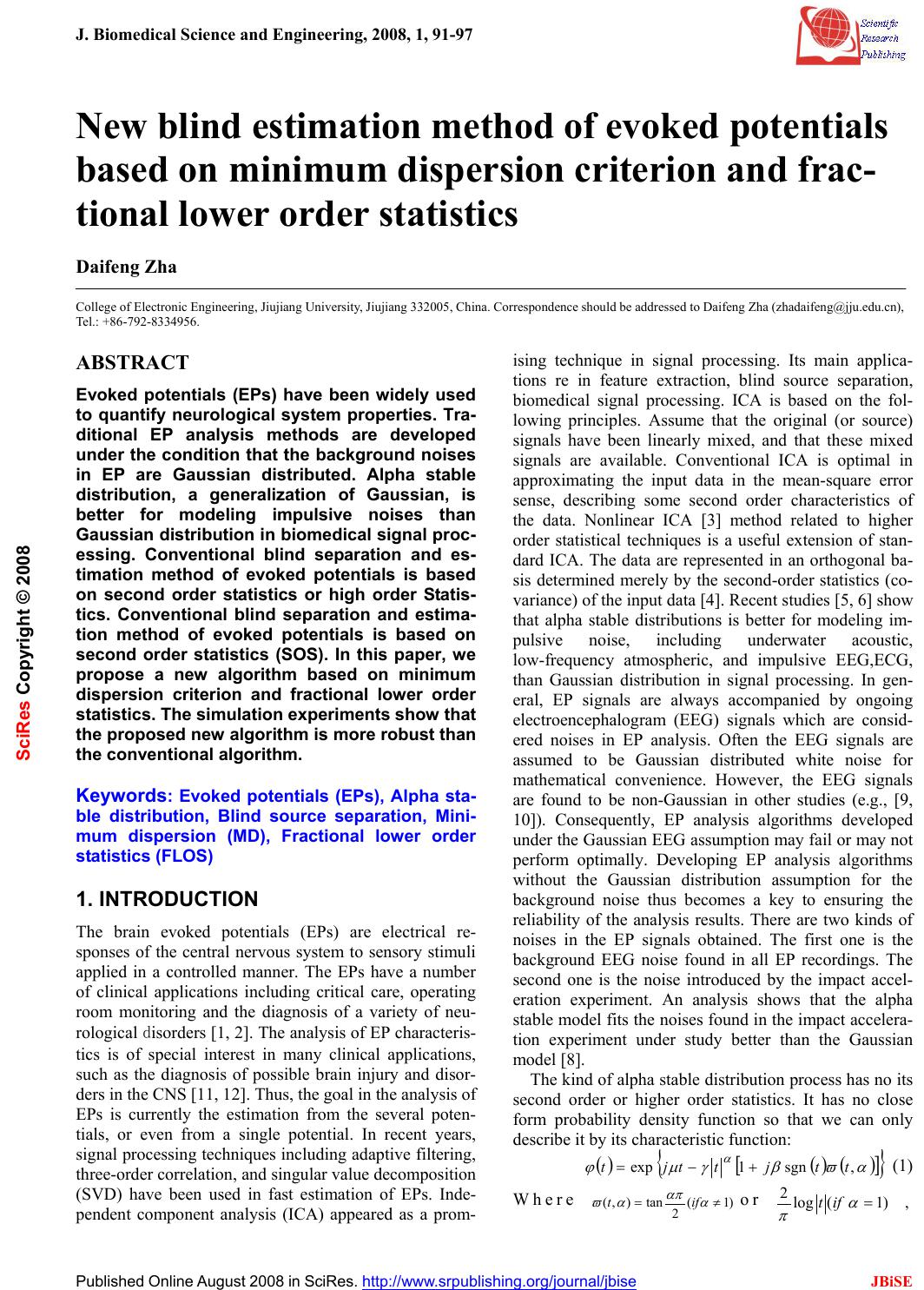J. Biomedical Science and Engineering, 2008, 1, 91-97
Published Online August 2008 in SciRes. http://www.srpublishing.org/journal/jbise JBiSE
New blind estimation method of evoked potentials
based on minimum dispersion criterion and frac-
tional lower order statistics
Daifeng Zha
College of Electronic Engineering, Jiujiang University, Jiujiang 332005, China. Correspondence should be addressed to Daifeng Zha ([e-mail]),
Tel.: [phone].
ABSTRACT
Evoked potentials (EPs) have been widely used
to quantify neurological system properties. Tra-
ditional EP analysis methods are developed
under the condition that the background noises
in EP are Gaussian distributed. Alpha stable
distribution, a generalization of Gaussian, is
better for modeling impulsive noises than
Gaussian distribution in biomedical signal proc-
essing. Conventional blind separation and es-
timation method of evoked potentials is based
on second order statistics or high order Statis-
tics. Conventional blind separation and estima-
tion method of evoked potentials is based on
second order statistics (SOS). In this paper, we
propose a new algorithm based on minimum
dispersion criterion and fractional lower order
statistics. The simulation experiments show that
the proposed new algorithm is more robust than
the conventional algorithm.
Keywords: Evoked potentials (EPs), Alpha sta-
ble distribution, Blind source separation, Mini-
mum dispersion (MD), Fractional lower order
statistics (FLOS)
1. INTRODUCTION
The brain evoked potentials (EPs) are electrical re-
sponses of the central nervous system to sensory stimuli
applied in a controlled manner. The EPs have a number
of clinical applications including critical care, operating
room monitoring and the diagnosis of a variety of neu-
rological disorders [1, 2]. The analysis of EP characteris-
tics is of special interest in many clinical applications,
such as the diagnosis of possible brain injury and disor-
ders in the CNS [11, 12]. Thus, the goal in the analysis of
EPs is currently the estimation from the several poten-
tials, or even from a single potential. In recent years,
signal processing techniques including adaptive filtering,
three-order correlation, and singular value decomposition
(SVD) have been used in fast estimation of EPs. Inde-
pendent component analysis (ICA) appeared as a prom-
ising technique in signal processing. Its main applica-
tions re in feature extraction, blind source separation,
biomedical signal processing. ICA is based on the fol-
lowing principles. Assume that the original (or source)
signals have been linearly mixed, and that these mixed
signals are available. Conventional ICA is optimal in
approximating the input data in the mean-square error
sense, describing some second order characteristics of
the data. Nonlinear ICA [3] method related to higher
order statistical techniques is a useful extension of stan-
dard ICA. The data are represented in an orthogonal ba-
sis determined merely by the second-order statistics (co-
variance) of the input data [4]. Recent studies [5, 6] show
that alpha stable distributions is better for modeling im-
pulsive noise, including underwater acoustic,
low-frequency atmospheric, and impulsive EEG,ECG,
than Gaussian distribution in signal processing. In gen-
eral, EP signals are always accompanied by ongoing
electroencephalogram (EEG) signals which are consid-
ered noises in EP analysis. Often the EEG signals are
assumed to be Gaussian distributed white noise for
mathematical convenience. However, the EEG signals
are found to be non-Gaussian in other studies (e.g., [9,
10]). Consequently, EP analysis algorithms developed
under the Gaussian EEG assumption may fail or may not
perform optimally. Developing EP analysis algorithms
without the Gaussian distribution assumption for the
background noise thus becomes a key to ensuring the
reliability of the analysis results. There are two kinds of
noises in the EP signals obtained. The first one is the
background EEG noise found in all EP recordings. The
second one is the noise introduced by the impact accel-
eration experiment. An analysis shows that the alpha
stable model fits the noises found in the impact accelera-
tion experiment under study better than the Gaussian
model [8].
The kind of alpha stable distribution process has no its
second order or higher order statistics. It has no close
form probability density function so that we can only
describe it by its characteristic function:
() () () []
{
}
αϖβγμϕ α ,sgn1exp ttjttjt +−= (1)
Where )1(
2
tan),( ≠= α
απ
αϖ ift or ,)1(log
2=
α
π
ift
SciRes Copyright © 2008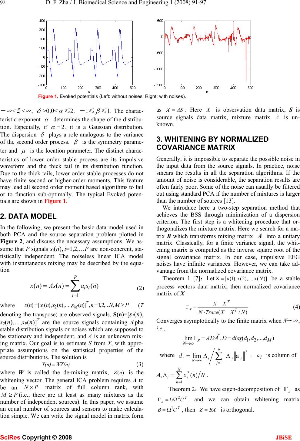

92 D. F. Zha / J. Biomedical Science and Engineering 1 (2008) 91-97
SciRes Copyright © 2008 JBiSE
Figure 1. Evoked potentials (Left: without noises; Right: with noises).
－∞<
ξ
<∞,
δ
>0,0<
α
≤2, －1≤
β
≤1. The charac-
teristic exponent
α
determines the shape of the distribu-
tion. Especially, if 2=
α
, it is a Gaussian distribution.
The dispersion
δ
plays a role analogous to the variance
of the second order process.
β
is the symmetry parame-
ter and
μ
is the location parameter. The distinct charac-
teristics of lower order stable process are its impulsive
waveform and the thick tail in its distribution function.
Due to the thick tails, lower order stable processes do not
have finite second or higher-order moments. This feature
may lead all second order moment based algorithms to fail
or to function sub-optimally. The typical Evoked poten-
tials are shown in Figure 1.
2. DATA MODEL
In the following, we present the basic data model used in
both PCA and the source separation problem plotted in
Figure 2, and discuss the necessary assumptions. We as-
sume that P signals si(n), i=1,2,…P are non-coherent, sta-
tistically independent. The noiseless linear ICA model
with instantaneous mixing may be described by the equa-
tion
∑
=
==
P
i
ii nsanAsnx
1
)()()( (2)
where PMNnnxnxnxnx T
M≥== ,,...2,1,)](),....,(),([)( 21 (T
denoting the transpose) are observed signals, S(n)=[s1(n),
s2(n),…,sP(n)]T are the source signals containing alpha
stable distribution signals or noises which are supposed to
be stationary and independent, and A is an unknown mix-
ing matrix. Our goal is to estimate S from X, with appro-
priate assumptions on the statistical properties of the
source distributions. The solution is
WZ(n)Y(n)= (3)
where W is called the de-mixing matrix, )(nZ is the
whitening vector. The general ICA problem requires A to
be an PN × matrix of full column rank, with
P
M
≥(i.e., there are at least as many mixtures as the
number of independent sources). In this paper, we assume
an equal number of sources and sensors to make calcula-
tion simple. We can write the signal model in matrix form
as ASX
=
. Here
X
is observation data matrix, S is
source signals data matrix, mixture matrix
A
is un-
known.
3. WHITENING BY NORMALIZED
COVARIANCE MATRIX
Generally, it is impossible to separate the possible noise in
the input data from the source signals. In practice, noise
smears the results in all the separation algorithms. If the
amount of noise is considerable, the separation results are
often fairly poor. Some of the noise can usually be filtered
out using standard PCA if the number of mixtures is larger
than the number of sources [13].
We introduce here a two-step separation method that
achieves the BSS through minimization of a dispersion
criterion. The first step is a whitening procedure that or-
thogonalizes the mixture matrix. Here we search for a ma-
trix B which transforms mixing matrix A into a unitary
matrix. Classically, for a finite variance signal, the whit-
ening matrix is computed as the inverse square root of the
signal covariance matrix. In our case, impulsive EEG
noises have infinite variances. However, we can take ad-
vantage from the normalized covariance matrix.
Theorem 1 [7]：Let )](x),...,2(x),1(x[X N= be a stable
process vectors data matrix, then normalized covariance
matrix of X
)/(
Γ
NXXTraceN
XX
T
T
x⋅
= (4)
Converges asymptotically to the finite matrix when
N →∞,
i.e.,
),...,,(,Γlim 21 M
T
x
N
ddddiagDADA ==
∞→
where 2
1
alim jj
P
j
i
N
i
dΔΔ=∑
=
∞→
，j a is column of
A,∑
=
=Δ
N
n
ii Nnx
1
2)(.
Theorem 2：We have eigen-decomposition of x
Γ as
T
xUU2
ΓΩ= and we can obtain whitening matrix
T
UB1 Ω= , then
B
X
Z
=
is orthogonal.

D. F. Zha / J. Biomedical Science and Engineering 1 (2008) 91-97 93
SciRes Copyright © 2008 JBiSE
Figure 2. Data and system model.
Proof：
TT
x
TTT/N)BTrace(XXNBΓBBXXZZ ⋅==
I/N)Trace(XXN
)(ΩIΩIΩ/N)Trace(XXN
)(ΩUUUΩUΩ/N)Trace(XXN
BUUΩB/N)Trace(XXN
T
T-12-1T
T-1T2T-1T
TT2T
⋅⋅=
⋅⋅⋅⋅⋅⋅⋅=
⋅⋅⋅⋅⋅=
⋅⋅⋅⋅=
So we can write
I))(BAD(BADBBADABBΓT1/21/2TTT
x=== and thus the
whitening of x(n) isBx(n)z(n) =.
4. DEMIXING ALGORITHM
The core part and most difficult task in BSS is learning of
the separating matrix W. During the last years, many neu-
ral blind separation algorithms have been proposed. In the
following, we discuss and propose separation algorithms
which are suitable for alpha stable noise environments in
PCA-type networks.
Let us consider ith output weight vector PiWi...2,1,
=
,
standard PCA is based on second order statistics and
maximize the output variances E{|yi(n)|2}=E{|Wi
TZ(n)|2}
subject to orthogonal constraintsPii IWW=
T. As lower
order alpha stable distribution noise has no second order
moment, we must select appropriate optimal criterion.
FLOS and related other statistics are clearly defined in [5,
6]. So we must use fractional lower order statistics (FLOS)
[5, 6], that is to say, the PCA problem corresponding to
p-order moment maximization is solution to optimization
problem. For each PiWi...2,1, =
) (}|W)(Z|
1
{maxarg T
WP
T
ii
p
i
opt
iIWWn
p
EW
i
== (5)
Let objective function be
∑≠=
+−+=
P
ijj
jiijiiii
p
ii n
p
EJ
,1
TT
TWW
2
1
)1WW(
2
1
}|W)(Z|
1
{)W( λλ
Here the Lagrange multiplier isij
λ
, imposed on the or-
thogonal constraints. For each neuron, i W is orthogonal
to the weight vectorij
j≠,W.
The estimated gradient of )(i JW with respect to i W
is
∑
=
−+=∇
P
j
jiji
p
ii WWnconjWnnZEWJ
1
T2T )})(Z(|)(Z|)({)(
ˆ
λ
(6)
At the optimum, the gradients must vanish for
Pi ,...2,1=, and ijj
T
i
WW δ =.These can be taken into ac-
count by multiplying (6) by T
j
Wfrom left. We can ob-
tain )}W)(Z(|W)(Z|)(Z{W T2T
T
i
p
ijijnconjnnE −
−= λ . In-
serting these into (6), we can get
)}W)(Z(|W)(Z|)(Z{]WWI[)W(
ˆT2T
1
T
i
p
i
P
j
jji nconjnnEJ −
=
∑
−=∇
(7)
A practical gradient algorithm for optimization problem
(5) is now obtained by inserting (7) into
))((
ˆ
)()()1(nJnnn iii WWW ∇−=+ μ ,
where )(n
μ
is the gain parameter. The final algorithm is
thus
|)(Z])(W)(WI)[()(W)1(W
1
Tnnnnnn
P
j
jjii∑
=
−−=+ μ
))(W)(Z(|)(W)(Z T2T nnconjnn i
p
i
− (8)
As )()()( Tnnnyii WZ=, (8) can be written as follow
))((|)(|)()(W)1(W 2nyconjnynnn i
p
iii
−
−=+ μ
])(W)()(Z[
1
∑
=
−
P
j
jjnnyn (9)
Let )(||)(2tconjttg p− =, then )(tg is appropriate PCA
network nonlinear transform function for lower order al-
pha stable distribution impulse noises.
Considering that during the iteration error item of gra-
dient ∑
=
−
P
j
T
jj nn
1
)()(WWI might be zero instantaneously,
we modify (9) in order to improve robustness of algorithm
as
])())(()())[(()()()1(
1
∑
=
−−=+
P
j
jiiiinnygnnygnnn WZWW
μ (10)
Thus P W,...,W,W 21 can be obtained.
Let Y(n)=[y1(n), y2(n), ..., yP(n)]T, W=[W1, W2, …, WP].
For whole network, solution to W and optimization
problem is
}|W(n)Z|
1
{maxargW T
1
W
opt
p
i
P
ip
E
∑
=
= (11)
According above derivation, by using
)(||)(2tconjttg p− =, the algorithm for learning W is thus
))(Y())](Y()(W)(Z)[()(W)1(W Tngngnnnnn −−=+ μ (12)
5. Performances Analysis
Different nonlinear function can be applied to different
blind signal separation problem. Many popular functions
are g(t)=sign(t) and g(t)=tanh(t) corresponding to thedou-
ble exponential distribution |)|exp(
2
1x−and the in-
verse-cosine-hyperbolic distribution)cosh(
11
x π
, re-
specttively. For the class of symmetric normal inverse

94 D. F. Zha / J. Biomedical Science and Engineering 1 (2008) 91-97
SciRes Copyright © 2008 JBiSE
Figure 3. The nonlinear function of alpha stable distribution.
Gaussian (NIG), it is straightforward to obtain according
to [14]
)(
)(
)( 22
1
22
2
22 tK
tK
t
t
tg
+
+
+
−
=
δα
δα
δ
α
, where K1(.) and
K2(.) are the modified Bessel function of the second kind
with index 1 and 2.
For lower order alpha stable distribution noise has no
second order or higher order moment, we must select
appropriate nonlinear function g(t)=| t |p-2 conj(t) (p <
α
).
If t is real data, then g(t)=| t |
p-1 sign(t). If p=1, then
g(t)=sign(t). Figure 3 shows the nonlinear function of
alpha stable distribution for different
α
.
We start from the learning rule (12), and we assume that
there exists a square separating matrix T
H such
that )()( TnnZHU =. The separating matrix H
T must be
orthogonal. To make the analysis easier, we multiply
both sides of the learning rule (12) byT
H. We obtain
))()(lg())]()(()(
)()[()()1(
nWnZnZnWgnWH
nZHnnWHnWH
TTT
TTT
−
+=+ μ
(13)
For the sake of P IHH =
T, we can get
))(WHH)(Z())](ZHH)(W()(WH
)(ZH)[()(WH)1(WH
TTTTT
TTT
nngnngn
nnnn −+=+ μ
(14)
Define )()(Tnn WHQ =,)(()( Tnn Q)HW-1 =, (14) is written as
))(U)(Q())](U)(Q()(Q
)(U)[()(Q)1(Q
TT nngnngn
nnnn−+=+
μ
(15)
Geometrically the transformation multiplying by the
orthogonal matrix T
Hsimply means a rotation to a new
set of coordinates such that the elements of the input
vector expressed in these coordinates are statistically
independent.
Analogous differential equation of (15) is obtained as
matrix form:
)}QU()UQ({)}QU(U{/Q TTT ggEgEdtd−= (16)
According to [15], we can easily prove that (16) has
stable solution. For the sake of Q=HTW, thus W=
(HT)-1Q is asymptotic stable solution of (12). Figure 4
shows the stability and convergence of algorithm based
on SOS and FLOS. From Figure 4, we know the algo-
rithm based on FLOS has better stability and conver-
gence than the algorithm based on SOS.
6. EXPERIMENTAL RESULTS
From Section I we know that the noise for EP could be a
lower order stable process. Through computer simula-
tions, we will demonstrate the effectiveness of the pro-
posed algorithm under alpha stable noise conditions. We
use correlation coefficient as follows to evaluate the per-
formances of the proposed algorithms:
∑∑∑ ===
=
N
n
j
N
n
i
N
n
jiji nynsnynsys
1
2
1
2
1
)()()()(),( τ (17)
Experiment 1
Two independent sources are linearly mixed. One is the
periodical noise free EP signal, and the period is 128
points, the sampling frequency is 1000Hz. The other is
an alpha stable non-Gaussian noise with7.1
=
α
. Two
algorithms are used in the experiment, including: (1)
SOS with nonlinear function )tanh()( ttg =;(2) FLOS
with )(||)(2tconjttg p− =，respectively. Figure 4 shows
the stability and convergence of algorithm based on SOS
and FLOS. We know the algorithm based on FLOS has
better stability and convergence than the algorithm based
on SOS.
We can get signals waveforms in time domain shown
in Figure 5, where (a) and (b) are source signals, (c) and
(d) are separated signals based on SOS, (e) and (f) are
separated signals based on FLOS. For FLOS algorithm,

D. F. Zha / J. Biomedical Science and Engineering 1 (2008) 91-97 95
SciRes Copyright © 2008 JBiSE
Figure 4. The stability and convergence.
Figure 5. Separating results: (a)-(b) are the source signals. (c)-(d) are the separated signals with SOS. (e)-(f) are the
separated signals with FLOS.
Figure 6. Separating results: (a)-(b) are the source signals. (c)-(d) are the separated signals with SOS. (e)-(f) are the
separated signals with FLOS.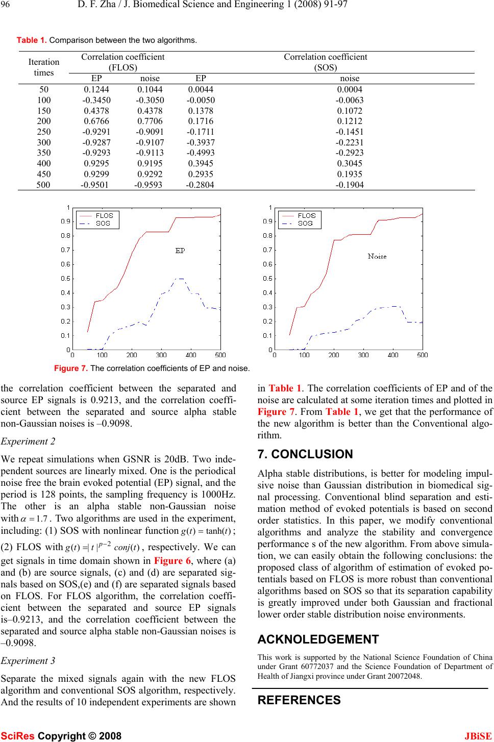

96 D. F. Zha / J. Biomedical Science and Engineering 1 (2008) 91-97
SciRes Copyright © 2008 JBiSE
Table 1. Comparison between the two algorithms.
Correlation coefficient
(FLOS)
Correlation coefficient
(SOS)
Iteration
times EP noise EP noise
50 0.1244 0.1044 0.0044 0.0004
100 -0.3450 -0.3050 -0.0050 -0.0063
150 0.4378 0.4378 0.1378 0.1072
200 0.6766 0.7706 0.1716 0.1212
250 -0.9291 -0.9091 -0.1711 -0.1451
300 -0.9287 -0.9107 -0.3937 -0.2231
350 -0.9293 -0.9113 -0.4993 -0.2923
400 0.9295 0.9195 0.3945 0.3045
450 0.9299 0.9292 0.2935 0.1935
500 -0.9501 -0.9593 -0.2804 -0.1904
Figure 7. The correlation coefficients of EP and noise.
the correlation coefficient between the separated and
source EP signals is 0.9213, and the correlation coeffi-
cient between the separated and source alpha stable
non-Gaussian noises is –0.9098.
Experiment 2
We repeat simulations when GSNR is 20dB. Two inde-
pendent sources are linearly mixed. One is the periodical
noise free the brain evoked potential (EP) signal, and the
period is 128 points, the sampling frequency is 1000Hz.
The other is an alpha stable non-Gaussian noise
with 7.1=
α
. Two algorithms are used in the experiment,
including: (1) SOS with nonlinear function)tanh()( ttg
=
;
(2) FLOS with)(||)( 2tconjttg p− =, respectively. We can
get signals in time domain shown in Figure 6, where (a)
and (b) are source signals, (c) and (d) are separated sig-
nals based on SOS,(e) and (f) are separated signals based
on FLOS. For FLOS algorithm, the correlation coeffi-
cient between the separated and source EP signals
is–0.9213, and the correlation coefficient between the
separated and source alpha stable non-Gaussian noises is
–0.9098.
Experiment 3
Separate the mixed signals again with the new FLOS
algorithm and conventional SOS algorithm, respectively.
And the results of 10 independent experiments are shown
in Table 1. The correlation coefficients of EP and of the
noise are calculated at some iteration times and plotted in
Figure 7. From Table 1, we get that the performance of
the new algorithm is better than the Conventional algo-
rithm.
7. CONCLUSION
Alpha stable distributions, is better for modeling impul-
sive noise than Gaussian distribution in biomedical sig-
nal processing. Conventional blind separation and esti-
mation method of evoked potentials is based on second
order statistics. In this paper, we modify conventional
algorithms and analyze the stability and convergence
performance s of the new algorithm. From above simula-
tion, we can easily obtain the following conclusions: the
proposed class of algorithm of estimation of evoked po-
tentials based on FLOS is more robust than conventional
algorithms based on SOS so that its separation capability
is greatly improved under both Gaussian and fractional
lower order stable distribution noise environments.
ACKNOLEDGEMENT
This work is supported by the National Science Foundation of China
under Grant 60772037 and the Science Foundation of Department of
Health of Jiangxi province under Grant 20072048.
REFERENCES

D. F. Zha / J. Biomedical Science and Engineering 1 (2008) 91-97 97
SciRes Copyright © 2008 JBiSE
[1] R. R. Gharieb, A. Cichocki. (2001) Noise reduction in brain evoked
potentials based on third-order correlations. IEEE Transactions on
Biomedical Engineering, 48(5): 501-512.
[2] C. E. Davila, R. Srebro, and I. A. Ghaleb. (1998) Optimal detection
of visual evoked potential. IEEE Transaction on Biomedical Engi-
neering, 45(6): 800–803.
[3] Yanwu Zhang,Yuanliang Ma (1997) CGHA for principal component
extraction in the complex domain. IEEE. Trans. on Neural Net-
work,vol 8,No.5.
[4] Mutihac, R. Van Hulle, M.M. (2003) PCA and ICA neural imple-
mentations for source separation - a comparative study. Proceedings
of the International Joint Conference on Neural Networks, Volume:
1 , 20-24.
[5] C. L. Nikias and M. shao. (1995) Signal Processing with Al-
pha-Stable Distributions and Applications. New York: John Wiley
& Sons Inc.
[6] M. shao and C. L. Nikias. (1993) Signal Processing with fractional
lower order moments: stable processes and their applications. Pro -
ceedings of IEEE, Vol.81, No.7, 986-1010.
[7] G. Samorodnitsky, M. S. Taqqu. (1994) Stable Non-Gaussian Ran-
dom Process: Stochastic Models with Infinite Variance. New York:
Chapman and Hall.
[8]Xuan Kong,Tianshuang Qiu. (1999) Adaptive Estimation of Latency
Change in Evoked Potentials by Direct Least Mean p-Norm
Time-Delay Estimation. IEEE Transactions on Biomedical Engi-
neering, vol. 46, No. 8, August.
[9] N. Hazarika, A. C. Tsoi, and A. A. Sergejew. (1997) Nonlinear
considerations in EEG signal classification. IEEE Trans. Signal
Processing, vol. 45, pp. 829–936.
[10] X. Ma and C. L. Nikias. (1996) Joint estimation of time delay and
frequency delay in impulsive noise using fractional lower-order sta-
tistics. IEEE Trans. Signal Processing, vol. 44, pp. 2669–2687, Nov.
[11] X. Kong and N. V. Thakor. (1996) Adaptive estimation of latency
changes in evoked potentials. IEEE Trans. Biomed. Eng., vol. 43, pp.
189–197, Feb.
[12] C. A. Vaz and N. V. Thakor. (1989) Adaptive Fourier estimation
of time varying evoked potentials. IEEE Trans. Biomed. Eng., vol.
36, pp. 448–455, Apr.
[13] Winter, S.; Sawada, H.; Makino, S. (2003) Geometrical under-
standing of the PCA subspace method for overdetermined blind
source separation.Acoustics, Speech, and Signal Processing.
[14] Preben Kidmose. (2001) Blind separation of heavy tail signals.
Technical university of denmark ,IMM-Phd, LYNGBY
[15] Juha Karhumen;Erkki Oja;Liuyue Wang;Ricardo Vigario;Jyrki
Joutsensalo. (1997) A class of neural networks for independent
component analysis. IEEE. Trans. on Neural Network,vol 8,No.3.