Applied Mathematics, 2011, 2, 890-898
doi:10.4236/am.2011.27119 Published Online July 2011 (http://www.SciRP.org/journal/am)
A Hybrid Optimization Technique Coupling an
Evolutionary and a Local Search Algorithm for Economic
Emission Load Dispatch Problem
A. A. Mousa, Kotb A. Kotb
Department of Mathematics and Statistics, Faculty of sciences, Taif University, Taif,
El-Haweiah, Kingdom of Saudi Arabia (KSA)
Received May 13, 2011; revised May 24, 2011; accepted May 27, 2011
Abstract
This paper presents an optimization technique coupling two optimization techniques for solving Economic
Emission Load Dispatch Optimization Problem EELD. The proposed approach integrates the merits of both
genetic algorithm (GA) and local search (LS), where it maintains a finite-sized archive of non-dominated
solutions which gets iteratively updated in the presence of new solutions based on the concept of
ε-dominance. To improve the solution quality, local search technique was applied as neighborhood search
engine, where it intends to explore the less-crowded area in the current archive to possibly obtain more non-
dominated solutions. TOPSIS technique can incorporate relative weights of criterion importance, which has
been implemented to identify best compromise solution, which will satisfy the different goals to some extent.
Several optimization runs of the proposed approach are carried out on the standard IEEE 30-bus 6-genrator
test system. The comparison demonstrates the superiority of the proposed approach and confirms its potential
to solve the multiobjective EELD problem.
Keywords: Economic Emission Load Dispatch, Evolutionary Algorithms, Multiobjective Optimization,
Local Search
1. Introduction
The purpose of EELD problem is to figure out the opti-
mal amount of the generated power for the fossil-based
generating units in the system by minimizing the fuel
cost and emission level simultaneously, subject to vari-
ous equality and inequality constraints including the se-
curity measures of the power transmission/distribution.
Different techniques have been reported in the litera-
ture pertaining to economic emission load dispatch pro-
blem. In [1,2] the problem has been reduced to a single
objective problem by treating the emission as a con-
straint with a permissible limit. This formulation, how-
ever, has a severe difficulty in getting the trade-off rela-
tions between cost and emission. Alternatively, minimiz-
ing the emission has been handled as another objective in
addition to usual cost objective. A linear programming
based optimization procedures in which the objectives
are considered one at a time was presented in [3]. Un-
fortunately, the EELD problem is a highly nonlinear and
a multimodal optimization problem. Therefore, conven-
tional optimization methods that make use of derivatives
and gradients, in general, not able to locate or identify
the global optimum. On the other hand, many mathe-
matical assumptions such as analytic and differential ob-
jective functions have to be given to simplify the prob-
lem. Furthermore, this approach does not give any in-
formation regarding the trade-offs involved.
In other research direction, the multiobjective EELD
problem was converted to a single objective problem by
linear combination of different objectives as a weighted
sum [4-7]. The important aspect of this weighted sum
method is that a set of Pareto-optimal solutions can be
obtained by varying the weights. Unfortunately, this re-
quires multiple runs as many times as the number of de-
sired Pareto-optimal solutions. Furthermore, this method
cannot be used to find Pareto-optimal solutions in prob-
lems having a nonconvex Pareto-optimal front. In addi-
tion, there is no rational basis of determining adequate
weights and the objective function so formed may lose

A. A. MOUSA ET AL.891
significance due to combining noncommensurable objec-
tives. To avoid this difficulty, the

-constraint method
for multiobjective optimization was presented in [8,9].
This method is based on optimization of the most pre-
ferred objective and considering the other objectives as
constraints bounded by some allowable levels. These
levels are then altered to generate the entire Pareto-optimal
set. The most obvious weaknesses of this approach are
that it is time-consuming and tends to find weakly non-
dominated solutions.
Goal programming method was also proposed for mul-
tiobjective EELD problem [10]. In this method, a target
or a goal to be achieved for each objective is assigned
and the objective function will then try to minimize the
distance from the targets to the objectives. Although the
method is computationally efficient, it will yield an infe-
rior solution rather than a noninferior one if the goal
point is chosen in the feasible domain. Hence, the main
drawback of this method is that it requires a priori know-
ledge about the shape of the problem search space.
Heuristic algorithms such as genetic algorithm have
been recently proposed for solving OPF problem [11-13].
The results reported were promising and encouraging for
further research. Moreover the studies on heuristic algo-
rithms over the past few years, have shown that these
methods can be efficiently used to eliminate most of dif-
ficulties of classical methods [14-18]. Since they are
population-based techniques, multiple Pareto-optimal
solutions can, in principle, be found in one single run.
In this paper a hybrid multiobjective approach is pro-
posed, which based on concept of co-evolution and re-
pair algorithm for handing constraints. ε-Dominance con-
cept was implemented to maintains a finite-sized archive
of non-dominated solutions which gets iteratively up-
dated according to the chosen ε-vector. TOPSIS [19]
approach has been implemented to select best compro-
mise solution, which will satisfy the different goals to
some extent. Also, LS method was introduced as neigh-
borhood search engine where it intends to explore the
less-crowded area in the current archive to possibly ob-
tain more nondominated solutions.
2. Multiobjective Optimization
Multiobjective optimization [11] differs from the single
objective case in several ways:
 The usual meaning of the optimum makes no sense in
the multiple objective case because the solution opti-
mizing all objectives simultaneously is, in general,
impractical; instead, a search is launched for a feasi-
ble solution yielding the best compromise among ob-
jectives on a set of, so called, efficient solutions;
 The identification of a best compromise solution re-
quires taking into account the preferences expressed
by the decision-maker;
 The multiple objectives encountered in real-life pro-
blems are often mathematical functions of contrasting
forms.
 A key element of a goal programming model is the
achievement function; that is, the function that meas-
ures the degree of minimization of the unwanted de-
viation variables of the goals considered in the model.
A general multiobjective optimization problem is ex-
pressed by:
 


T
12
T
12
min ,,,
s.t.
,,,
m
n
F
xfxfxfx
xS
xxx x





where






12
,,,
m
f
xfxfxare the m objectives func-
tions,


12
,,,
n
x
xx
n SR
are the n optimization parameters,
and is the solution or parameter space.
Definition 1. (Pareto optimal solution ): *
x
is said to
be a Pareto optimal solution of MOP if there exists no other
feasible
x
(i.e.,
x
S

) such that,



*
jj
f
xfx
for
all 1, ,jm2,

 and


j

*
j
f
xfx
for at least one
objective function
j
f
.
Definition 2 [20]. (ε-dominance) Let :m
f
xR and
,ab X

. Then is said to ε-dominate for some ε
> 0, denoted as , if and only if for
ab
ab




im1, ,






1ii
f
afb 
According to Definition 2, the ε value stands for a
relative “tolerance” allowed for the objective values
which declared in Figure 1. This is especially important
in higher dimensional objective spaces, where the con-
cept of ε-dominance can reduce the required number of
solutions considerably. Also, the use of

-dominance
also makes the algorithms practical by allowing a deci-
sion maker to control the resolution of the Pareto set ap-
proximation by choosing an appropriate

value.
3. Economic Emission Load Dispatch
(EELD)
The economic emission load dispatch involves the si-
multaneous optimization of fuel cost and emission object-
Figure 1. Graphs visualizing the concepts of dominance (left)
and ε-dominance (right).

A. A. MOUSA ET AL. 892
tives which are conflicting ones. The deterministic prob-
lem is formulated as described below.
3.1. Objective Functions
Fuel Cost Objective. The classical economic dispatch
problem of finding the optimal combination of power
generation, which minimizes the total fuel cost while
satisfying the total required demand can be mathemati-
cally stated as follows [9]:



2
11
()$ hr
nn
tiGi iiGiiGi
ii
fC CPabPcP

 

where
: total fuel cost ($/hr), : is fuel cost of generator
,,: fuel cost coefficients of generator ,
i
iii
CC
abc i
i
: power generated (.)by generator ,
: number of generator.
Gi
Ppu
n
i
Emission Objective. The emission function can be
presented as the sum of all types of emission considered,
such as
N
O
x
,2 SO , thermal emission, etc., with suitable
pricing or weighting on each pollutant emitted. In the
present study, only one type of emission
N
O
x
is taken
into account without loss of generality. The amount of
N
O
x
emission is given as a function of generator output,
that is, the sum of a quadratic and exponential function:


2
22
1
()
10expton hr
x
NO
n
iiGi iGiiiGi
i
fE
PP P  







where, ,,,,
iiiii

 : coefficients of the i th genera-
tor’s
N
O
x
emission characteristic.
3.2. Constraints
The optimization problem is bounded by the following
constraints:
 Power balance constraint. The total power gener-
ated must supply the total load demand and the
transmission losses.
1
0
n
Gi D Loss
i
PPP

 

where
D
P: total load demand (p.u.), and : trans-
mission losses (p.u.).
loss
P
The transmission losses are given by [21]:

11
nn
Lossij ijijijijij
ii
PAPPQQBQPP






Q

where
 
, Q,
Acos, Bsin
iGi DiiGiDi
ij ij
ijij ijij
ij ij
PP PQQ
RR
VV VV


 

n: number of buses
ij
R
V
: series resistance connecting buses i and j
i: voltage magnitude at bus i
i

: voltage angle at bus i
i
Q
P: real power injection at bus i
: reactive power injection at bus i
 Maximum and Minimum Limits of Power Gen-
eration. The power generated Gi
P by each generator
is constrained between its minimum and maximum
limits, i.e.,
minmax minmax
min max
, ,
, 1,,
GiGi GiGiGiGi
iii
PPP QQQ
VVVi n
 
 
where minGi : minimum power generated, and :
maximum power generated.
PmaxGi P
 Security Constraints. A mathematical formulation
of the security constrained EELD problem would re-
quire a very large number of constraints to be consid-
ered. However, for typical systems the large propor-
tion of lines has a rather small possibility of becom-
ing overloaded. The EELD problem should consider
only the small proportion of lines in violation, or near
violation of their respective security limits which are
identified as the critical lines. We consider only the
critical lines that are binding in the optimal solution.
The detection of the critical lines is assumed done by
the experiences of the DM. An improvement in the
security can be obtained by minimizing the following
objective function.
 

max
1
k
GijGj
j
SfPTP T



where,


j
G
TP is the real power flow is the
maximum limit of the real power flow of the jth line and
k is the number of monitored lines. The line flow of the
jth line is expressed in terms of the control variables Gs,
by utilizing the generalized generation distribution fac-
tors (GGDF) [22] and is given below.
max
j
T
P
 
1
n
J
Gji
i
TP DP

Gi
where,
j
i is the generalized GGDF for line j, due to
generator i.
D
For secure operation, the transmission line loading
is restricted by its upper limit as
l
S
max ,1,,SS n


 
where is the number of transmission line. n
 
3.3. Multiobjective Formulation of EELD
Problem
The multiobjective EELD optimization problem [11] is

A. A. MOUSA ET AL.893
therefore formulated as:



1
2
1
2
22
1
1
max
()
$
()
10exp
s.t. 0,
,
x
t
n
iiGiiGi
i
NO
n
iiGi iGiiiGi
i
n
Gi D Loss
i
MinfxC
abP cPhr
Min fE
PPPton hr
PPP
SS
 










 





min max
min max
min max
1,,,
1,,
1,,
1,,
Line
GiGi Gi
GiGi Gi
iii
n
PPPi n
QQQi n
VVVi n

 
 
 






4. The Proposed Algorithm
Recently, the studies on evolutionary algorithms have
shown that these algorithms can be efficiently used to
eliminate most of the difficulties of classical methods
which can be summarized as:
 An algorithm has to be applied many times to find
multiple Pareto-optimal solutions.
 Most algorithms demand some knowledge about the
problem being solved.
 Some algorithms are sensitive to the shape of the
Pareto-optimal front.
 The spread of Pareto-optimal solutions depends on
efficiency of the single objective optimizer.
It is worth mentioning that the goal of a multiobjective
optimization problem is not only guide the search to-
wards Pareto-optimal front but also maintain population
diversity.
4.1. Initialization Stage
The algorithm uses two separate population [11], the first
population consists of the individuals which ini-
tialized randomly satisfying the search space (The lower
and upper bounds), while the second population
consists of reference points which satisfying all con-
straints. However, in order to ensure convergence to the
true Pareto-optimal solutions, we concentrated on how
elitism could be introduced in the algorithm. So, we pro-
pose an archiving/selection [20] strategy that guarantees
at the same time progress towards the Pareto-optimal set
and a covering of the whole range of the non-dominated
solutions. The algorithm maintains an externally fi-
nite-sized archive

t
P

t
R

t
A
of non-dominated solutions which
gets iteratively updated in the presence of new solutions
based on the concept of

-dominance.
4.2. Repair Algorithm
The idea of this technique [11] is to separate any feasible
individuals in a population from those that are infeasible
by repairing infeasible individuals. This approach co-
evolves the population of infeasible individuals until they
become feasible. Repair process works as follows. As-
sume, there is a search point S


rS
(where is the
feasible space). In such a case the algorithm selects one
of the reference points (Better reference point has better
chances to be selected), say and creates random
points
S
Z
from the segment defined between , r

, but
the segment may be extended equally on both sides de-
termined by a user specified parameter


0,  1. Thus, a
new feasible individual is expressed as:


12
1, 1zrz r

 


where


12

 

 and


0, 1   is a random
generated number
4.3. LS Stage
In this stage, we present modified local search technique
(MLS) [23] to improve the solution quality and to ex-
plore the less-crowded area in the external archive to
possibly obtain more nondominated solutions nearby.
We propose a MLS, which is a modification of Hooke
and Jeeves method [24] to be suitable for MOP. The
general procedure of the MLS techniques can be de-
scribed by the following steps.
Step 1. Start with an arbitrarily chosen point


n
m
t
X
E

, and the prescribed step lengths i
x

in
each of the coordinate directions i Set m
= 0, assume that m is the size of .
,1,2,,ui
t
.n
E
Step 2. Set m = m + 1, and k = 1 where k is number of
trial (s.t., max 1, ,kk

) to obtain preferred solution than
m
X
.
Step 3. The variable i
x
is perturbed about the current
temporary base point m
X
to obtain the new temporary
base point m
X

as :

 

 

1,2,,
m
mii
mii
m
X
Xxuifff
Xxuiffffi
Xiffff



n


 

  







where,




m
ffX ,

 
mii
f
fX xu
 , and




mii
f
fX xu
 . Assume



f
is the evaluation of
the objective functions at a point.
Step 4. If the point m
X
unchanged.
While the number of trial k not satisfied, reduce the
step length i
x

. The following dynamic equation is
presented to reduce i
x

,

A. A. MOUSA ET AL. 894
 
max
1, 0,1
k
k
ii
xx rr




and go to step 3.
Step 5. Else, if m
X
 is preferred than m
X
(i.e.,
 
mm
f
XfX
) ,then m
X
is the new base point.
Step 6. With the help of the base points m
X
 m and
X

,
blish a pattern direction S as esta
mm
SX X


and find a point m
X
 as λS
mm
XX



, where

is
the step length, (taken as 1).
Step 7. If
 
mm

f
XfX
 
 set mm
X
X
, mm
X
X



,
and go to 6.
Step 8. If
 
mm

f
XfX
 

 set mm
X
X , and go to
4.
These steps is implemented on all nondominated solu-
tions in t
A
to get the true Pareto optimal solution and to
explore the less-crowded area in the external archive.
Figure 2 shows the pseudo code of the MLS algorithm.
4.4. Identifying a Best Compromise Solution
Optimization of the above-formulated objective func-
tions [11] yields not a single optimal solution, but a set
of Pareto optimal solutions, in which one objective can-
not be improved without sacrificing other objectives. For
practical applications, however, we need to select one
solution, which will satisfy the different goals to some
extent. Such a solution is called best compromise solu-
tion. TOPSIS method given by Yoon and Hwang [19]
has the ability to identify the best alternative from a fi-
nite set of alternatives quickly. It stands for “Technique
for Order Preference by Similarity to the Ideal Solution”
which based upon the concept that the chosen alternative
should have the shortest distance from the positive ideal
solution and the farthest from the negative ideal solution.
MLS technique
Start with
t
m
XE
Generate
m
X
While (
 
m
fX fX
m
stopped criterion satisfied) DO
If
mm
XX

Reduce Generate
i
x m X
End
Establish a pattern direction Generate Sm X
If

mm
f
XfX

, set ,
mm
XX

mm XX


Set Generate
Sm X
Else if  
mm
f
XfX
 

mm
XX


End
End
Figure 2. The pseudo code of the MLS algorithm.
TOPSIS can incorporate relative weights of criterion
importance. The idea of TOPSIS can be expressed in a
series of steps.
Step1: Obtain performance data for n alternatives over
M criteria ij
x


1, ,,1, ,injM.
Step2: Calculate normalized rating (vector normaliza-
tion is used) .
ij
Step3: Develop a set of importance weights
r
j
W, for
each of the criteria. The basis for these weights can be
anything, but, usually, is adhoc reflective of relative im-
portance.
ijj ij
Vwr


Step4: Identify the ideal alternative (extreme per-
formance on each criterion) . S




1
12
,,,,
max, min,1,,
jm
ij ij
Sv v v
vj Jvj Jin
  

 



where!
J
is a set of benefit attributes and2
J
is a set
of cost attributes.
Step5: Identify the nadir alternative (reverse extreme
performance on each criterion) . S




1
12
,,,,
min ,max ,1,,
jm
ij ij
Sv v v
vj Jvj Jin


 



Step6: Develop a distance measure over each criterion
to both ideal (D

) and nadir (). D
 
_
22
,
i ijji ijj
jj
DvvDvv

 



Step7: For each alternative, determine a ratio R equal
to the distance to the nadir divided by the sum of the
distance to the nadir and the distance to the ideal,
D
RDD



Step8: Rank alternative according to ratio R (in Step 7)
in descending order, recommend the alternative with the
maximum ratio. The pseudo code of the proposed algo-
rithm are shown in Figure 3.
4.5. Basic Algorithm
It uses two separate population, the first population

0t
P

(where t is the iteration counter) consists of the
individuals which initialized randomly satisfying the
search space, while the second population consists
of reference points which satisfying all constraints. Also,
it stores initially the Pareto-optimal solutions externally
in a finite sized archive of non-dominated solutions

t
R

0
A
.
We use cluster algorithm to create the next population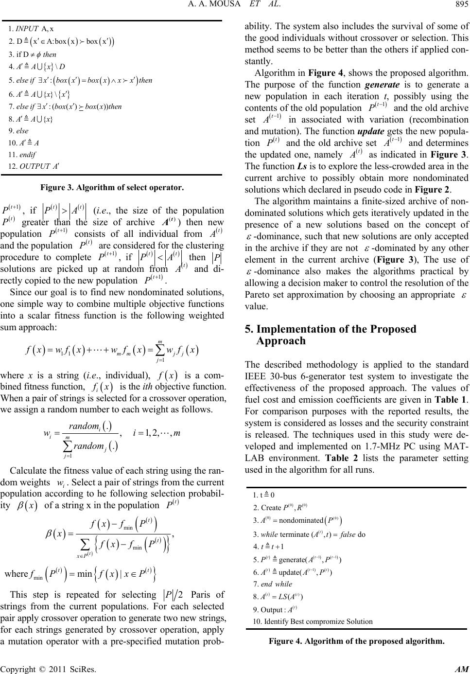

A. A. MOUSA ET AL.895
  

  

1. A,x
2. DxA:boxxboxx
3. if D
4. \
5. :
6. {}\
7. :(()())
8. {}
9.
10.
11.
12.
INPUT
then
AA xD
else ifxboxxboxxxxthen
AAxx
else ifxboxxboxxthen
AAx
else
AA
endif
OUTPUT A





  

 










Figure 3. Algorithm of select operator.

1t
P, if
 
t
PAt (i.e., the size of the population
greater than the size of archive ) then new
population consists of all individual from

t
P()t A

1t
P

t
A
and the population are considered for the clustering
procedure to complete

, if

t
P

1t
P
 
t
At P then P
solutions are picked up at random from

t
A
and di-
rectly copied to the new population .

1t
P
Since our goal is to find new nondominated solutions,
one simple way to combine multiple objective functions
into a scalar fitness function is the following weighted
sum approach:
 
11
1
m
mmj j
j
f
xwfxwfxwfx

 


where x is a string (i.e., individual),

f
x is a com-
bined fitness function,

i
f
x is the ith objective function.
When a pair of strings is selected for a crossover operation,
we assign a random number to each weight as follows.


1
., 1,2,,
.
i
im
j
j
random
wi
random



m
Calculate the fitness value of each string using the ran-
dom weights i. Select a pair of strings from the current
population according to he following selection probabil-
ity

w
x
 oing x in the population

t
P f a str
 




 

min
min
,
t
t
t
xP
fx fP
x
fx fP










min
where min|
tt
fP fxxP
This step is repeated for selecting 2P Paris of
strings from the current populations. For each selected
pair apply crossover operation to generate two new strings,
for each strings generated by crossover operation, apply
a mutation operator with a pre-specified mutation prob-
ability. The system also includes the survival of some of
the good individuals without crossover or selection. This
method seems to be better than the others if applied con-
stantly.
Algorithm in Figure 4, shows the proposed algorithm.
The purpose of the function generate is to generate a
new population in each iteration t, possibly using the
contents of the old population and the old archive
set

1t
P

1t
A

in associated with variation (recombination
and mutation). The function update gets the new popula-
tion and the old archive set

t
P

1t
A
 and determines
the updated one, namely

t
A
as indicated in Figure 3.
The function Ls is to explore the less-crowded area in the
current archive to possibly obtain more nondominated
solutions which declared in pseudo code in Figure 2.
The algorithm maintains a finite-sized archive of non-
dominated solutions which gets iteratively updated in the
presence of a new solutions based on the concept of

-dominance, such that new solutions are only accepted
in the archive if they are not

-dominated by any other
element in the current archive (Figure 3), The use of

-dominance also makes the algorithms practical by
allowing a decision maker to control the resolution of the
Pareto set approximation by choosing an appropriate

value.
5. Implementation of the Proposed
Approach
The described methodology is applied to the standard
IEEE 30-bus 6-generator test system to investigate the
effectiveness of the proposed approach. The values of
fuel cost and emission coefficients are given in Table 1.
For comparison purposes with the reported results, the
system is considered as losses and the security constraint
is released. The techniques used in this study were de-
veloped and implemented on 1.7-MHz PC using MAT-
LAB environment. Table 2 lists the parameter setting
used in the algorithm for all runs.
 



 
 


00
0(0)
11
1
()
1. t0
2. Create ,
3. nondominated
3. terminate (,) do
4. 1
5. generate(,)
6. update(,)
7.
8. ()
9. Output:
10. Identify Best comprom
t
ttt
ttt
tt
t
PR
AP
whileA tfalse
tt
PAP
AAP
end while
ALSA
A










ize Solution
Figure 4. Algorithm of the proposed algorithm.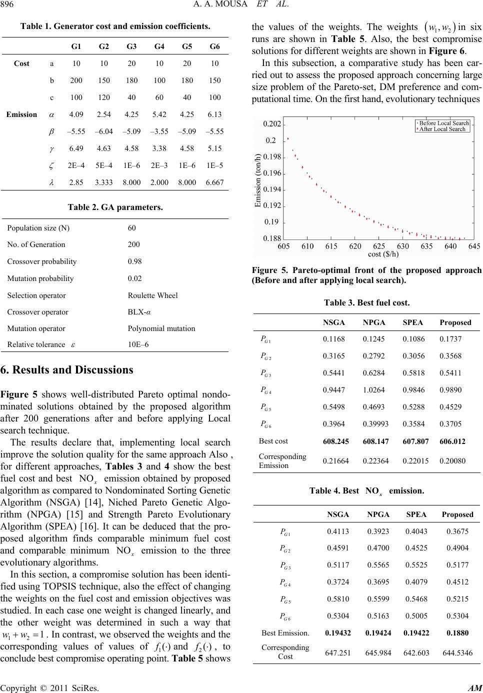

A. A. MOUSA ET AL. 896
Table 1. Generator cost and emission coefficients.
G1 G2 G3 G4 G5 G6
Cost a 10 10 20 10 20 10
b 200 150 180 100 180 150
c 100 120 40 60 40 100
Emission

4.09 2.54 4.25 5.42 4.25 6.13

–5.55 –6.04 –5.09 –3.55 –5.09 –5.55

6.49 4.63 4.58 3.38 4.58 5.15

2E–4 5E–4 1E–6 2E–3 1E–6 1E–5

2.85 3.333 8.000 2.000 8.000 6.667
Table 2. GA parameters.
Population size (N) 60
No. of Generation 200
Crossover probability 0.98
Mutation probability 0.02
Selection operator Roulette Wheel
Crossover operator BLX-α
Mutation operator Polynomial mutation
Relative tolerance

10E–6
6. Results and Discussions
Figure 5 shows well-distributed Pareto optimal nondo-
minated solutions obtained by the proposed algorithm
after 200 generations after and before applying Local
search technique.
The results declare that, implementing local search
improve the solution quality for the same approach Also ,
for different approaches, Tables 3 and 4 show the best
fuel cost and best
N
O
x
emission obtained by proposed
algorithm as compared to Nondominated Sorting Genetic
Algorithm (NSGA) [14], Niched Pareto Genetic Algo-
rithm (NPGA) [15] and Strength Pareto Evolutionary
Algorithm (SPEA) [16]. It can be deduced that the pro-
posed algorithm finds comparable minimum fuel cost
and comparable minimum
N
O
x
emission to the three
evolutionary algorithms.
In this section, a compromise solution has been identi-
fied using TOPSIS technique, also the effect of changing
the weights on the fuel cost and emission objectives was
studied. In each case one weight is changed linearly, and
the other weight was determined in such a way that
12. In contrast, we observed the weights and the
corresponding values of values of1and 2
1ww
()f ()
f

, to
conclude best compromise operating point. Table 5 shows
the values of the weights. The weights in six
runs are shown in Table 5. Also, the best compromise
solutions for different weights are shown in Figure 6.

12
,ww

In this subsection, a comparative study has been car-
ried out to assess the proposed approach concerning large
size problem of the Pareto-set, DM preference and com-
putational time. On the first hand, evolutionary techniques
Figure 5. Pareto-optimal front of the proposed approach
(Before and after applying local search).
Table 3. Best fuel cost.
NSGA NPGA SPEA Proposed
1G
P 0.1168 0.1245 0.1086 0.1737
2G
P 0.3165 0.2792 0.3056 0.3568
3G
P 0.5441 0.6284 0.5818 0.5411
4G
P 0.9447 1.0264 0.9846 0.9890
5G
P 0.5498 0.4693 0.5288 0.4529
6G
P 0.3964 0.39993 0.3584 0.3705
Best cost 608.245 608.147 607.807 606.012
Corresponding
Emission 0.21664 0.22364 0.22015 0.20080
Table 4. Best emission. NOx
NSGA NPGA SPEA Proposed
1G
P 0.4113 0.3923 0.4043 0.3675
2G
P 0.4591 0.4700 0.4525 0.4904
3G
P 0.5117 0.5565 0.5525 0.5177
4G
P 0.3724 0.3695 0.4079 0.4512
5G
P 0.5810 0.5599 0.5468 0.5215
6G
P 0.5304 0.5163 0.5005 0.5304
Best Emission. 0.194320.19424 0.19422 0.1880
Corresponding
Cost 647.251645.984 642.603 644.5346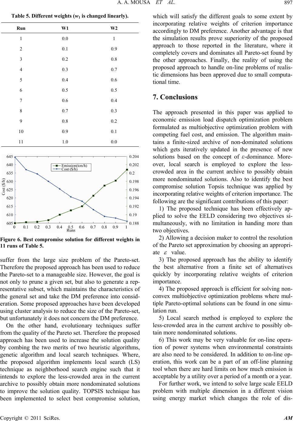

A. A. MOUSA ET AL.897
Table 5. Different weights (w1 is changed linearly).
W2 W1 Run
1 0.0 1
0.9 0.1 2
0.8 0.2 3
0.7 0.3 4
0.6 0.4 5
0.5 0.5 6
0.4 0.6 7
0.3 0.7 8
0.2 0.8 9
0.1 0.9 10
0.0 1.0 11
Figure 6. Best compromise solution for different weights in
11 runs of Table 5.
suffer from the large size problem of the Pareto-set.
Therefore the proposed approach has been used to reduce
the Pareto-set to a manageable size. However, the goal is
not only to prune a given set, but also to generate a rep-
resentative subset, which maintains the characteristics of
the general set and take the DM preference into consid-
eration. Some proposed approaches have been developed
using cluster analysis to reduce the size of the Pareto-set,
but unfortunately it does not concern the DM preference.
On the other hand, evolutionary techniques suffer
from the quality of the Pareto set. Therefore the proposed
approach has been used to increase the solution quality
by combing the two merits of two heuristic algorithms,
genetic algorithm and local search techniques. Where,
the proposed algorithm implements local search (LS)
technique as neighborhood search engine such that it
intends to explore the less-crowded area in the current
archive to possibly obtain more nondominated solutions
to improve the solution quality. TOPSIS technique has
been implemented to select best compromise solution,
which will satisfy the different goals to some extent by
incorporating relative weights of criterion importance
accordingly to DM preference. Another advantage is that
the simulation results prove superiority of the proposed
approach to those reported in the literature, where it
completely covers and dominates all Pareto-set found by
the other approaches. Finally, the reality of using the
proposed approach to handle on-line problems of realis-
tic dimensions has been approved due to small computa-
tional time.
7. Conclusions
The approach presented in this paper was applied to
economic emission load dispatch optimization problem
formulated as multiobjective optimization problem with
competing fuel cost, and emission. The algorithm main-
tains a finite-sized archive of non-dominated solutions
which gets iteratively updated in the presence of new
solutions based on the concept of ε-dominance. More-
over, local search is employed to explore the less-
crowded area in the current archive to possibly obtain
more nondominated solutions. Also to identify the best
compromise solution Topsis technique was applied by
incorporating relative weights of criterion importance. The
following are the significant contributions of this paper:
1) The proposed technique has been effectively ap-
plied to solve the EELD considering two objectives si-
multaneously, with no limitation in handing more than
two objectives.
2) Allowing a decision maker to control the resolution
of the Pareto set approximation by choosing an appropri-
ate

value.
3) The proposed approach has the ability to identify
the best alternative from a finite set of alternatives
quickly by incorporating relative weights of criterion
importance.
4) The proposed approach is efficient for solving non-
convex multiobjective optimization problems where mul-
tiple Pareto-optimal solutions can be found in one simu-
lation run.
5) Local search method is employed to explore the
less-crowded area in the current archive to possibly ob-
tain more nondominated solutions.
6) This work may be very valuable for on-line opera-
tion of power systems when environmental constraints
are also need to be considered. In addition to on-line op-
eration, this work can be a part of an off-line planning
tool when there are hard limits on how much emission is
acceptable by a utility over a period of a month or a year.
For further work, we intend to solve large scale EELD
problem with multiple dimension in a different vision
using energy market which changes the role of dis-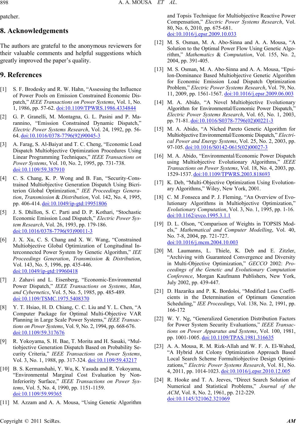

A. A. MOUSA ET AL. 898
patcher.
8. Acknowledgements
The authors are grateful to the anonymous reviewers for
their valuable comments and helpful suggestions which
greatly improved the paper’s quality.
9. References
[1] S. F. Brodesky and R. W. Hahn, “Assessing the Influence
of Power Pools on Emission Constrained Economic Dis-
patch,” IEEE Transactions on Power Systems, Vol. 1, No.
1, 1986, pp. 57-62. doi:10.1109/TPWRS.1986.4334844
[2] G. P. Granelli, M. Montagna, G. L. Pasini and P. Ma-
rannino, “Emission Constrained Dynamic Dispatch,”
Electric Power Systems Research, Vol. 24, 1992, pp. 56-
64. doi:10.1016/0378-7796(92)90045-3
[3] A. Farag, S. Al-Baiyat and T. C. Cheng, “Economic Load
Dispatch Multiobjective Optimization Procedures Using
Linear Programming Techniques,” IEEE Transactions on
Power Systems, Vol. 10, No. 2, 1995, pp. 731-738.
doi:10.1109/59.387910
[4] C. S. Chang, K. P. Wong and B. Fan, “Security-Cons-
trained Multiobjective Generation Dispatch Using Bicri-
terion Global Optimization,” IEE Proceedings Genera-
tion, Transmission & Distribution, Vol. 142, No. 4, 1995,
pp. 406-414. doi:10.1049/ip-gtd:19951806
[5] J. S. Dhillon, S. C. Parti and D. P. Kothari, “Stochastic
Economic Emission Load Dispatch,” Electric Power Sys-
tem Research, Vol. 26, 1993, pp. 179-186.
doi:10.1016/0378-7796(93)90011-3
[6] J. X. Xu, C. S. Chang and X. W. Wang, “Constrained
Multiobjective Global Optimization of Longitudinal In-
terconnected Power System by Genetic Algorithm,” IEE
Proceedings Generation, Transmission & Distribution,
Vol. 143, No. 5, 1996, pp. 435-446.
doi:10.1049/ip-gtd:19960418
[7] J. Zahavi and L. Eisenberg, “Economic-Environmental
Power Dispatch,” IEEE Transactions on Systems, Man,
and Cybernetics, Vol. 5, No. 5, 1985, pp. 485-489.
doi:10.1109/TSMC.1975.5408370
[8] Y. T. Hsiao, H. D. Chiang, C. C. Liu and Y. L. Chen, “A
Computer Package for Optimal Multi-Objective VAR
Planning in Large Scale Power Systems,” IEEE Transac-
tions on Power Systems, Vol. 9, No. 2, 1994, pp. 668-676.
doi:10.1109/59.317676
[9] R. Yokoyama, S. H. Bae, T. Morita and H. Sasaki, “Mul-
tiobjective Generation Dispatch Based on Probability Se-
curity Criteria,” IEEE Transactions on Power Systems,
Vol. 3, No. 1, 1988, pp. 317-324. doi:10.1109/59.43217
[10] B. S. Kermanshahi, Y. Wu, K. Yasuda and R. Yokoyama,
“Environmental Marginal Cost Evaluation by Non-
Inferiority Surface,” IEEE Transactions on Power Sys-
tems, Vol. 5, No. 4, 1990, pp. 1151-1159.
doi:10.1109/59.99365
[11] M. Azzam and A. A. Mousa, “Using Genetic Algorithm
and Topsis Technique for Multiobjective Reactive Power
Compensation,” Electric Power Systems Research, Vol.
80, No. 6, 2010, pp. 675-681.
doi:10.1016/j.epsr.2009.10.033
[12] M. S. Osman, M. A. Abo-Sinna and A. A. Mousa, “A
Solution to the Optimal Power Flow Using Genetic Algo-
rithm,” Mathematics & Computation, Vol. 155, No. 2,
2004, pp. 391-405.
[13] M. S. Osman, M. A. Abo-Sinna and A. A. Mousa, “Epsi-
lon-Dominance Based Multiobjective Genetic Algorithm
for Economic Emission Load Dispatch Optimization
Problem,” Electric Power Systems Research, Vol. 79, No.
11, 2009, pp. 1561-1567. doi:10.1016/j.epsr.2009.06.003
[14] M. A. Abido, “A Novel Multiobjective Evolutionary
Algorithm for Environmental/Economic Power Dispatch,”
Electric Power Systems Research, Vol. 65, No. 1, 2003,
pp. 71-81. doi:10.1016/S0378-7796(02)00221-3
[15] M. A. Abido, “A Niched Pareto Genetic Algorithm for
Multiobjective Environmental/Economic Dispatch,” Electri-
cal Power and Energy Systems, Vol. 25, No. 2, 2003, pp.
97-105. doi:10.1016/S0142-0615(02)00027-3
[16] M. A. Abido, “Environmental/Economic Power Dispatch
using Multiobjective Evolutionary Algorithms,” IEEE
Transactions on Power Systems, Vol. 18, No. 4, 2003, pp.
1529-1537. doi:10.1109/TPWRS.2003.818693
[17] K. Deb, “Multi-Objective Optimization Using Evolution-
ary Algorithms,” Wiley, New York, 2001.
[18] C. M .Fonseca and P. J. Fleming, “An Overview of Evo-
lutionary Algorithms in Multiobjective Optimization,”
Evolutionary Computation, Vol. 3, No. 1, 1995, pp. 1-16.
doi:10.1162/evco.1995.3.1.1
[19] D. L. Olson, “Comparison of Weights in TOPSIS Mod-
els,” Mathematical and Computer Modelling, Vol. 40,
No. 7-8, 2004, pp. 721-727.
doi:10.1016/j.mcm.2004.10.003
[20] M. Laumanns, L. Thiele, K. Deb and E. Zitzler,
“Archiving with Guaranteed Convergence and Diversity
in Multi-Objective Optimization,” GECCO 2002: Pro-
ceedings of the Genetic and Evolutionary Computation
Conference, Morgan Kaufmann Publishers, New York,
July 2002, pp. 439-447.
[21] D. Hazarika and P. K. Bordoloi, “Modified Loss Coeffi-
cients in the Determination of Optimum Generation
Scheduling,” IEE Proceedings, Vol. 138, No. 2, 1991, pp.
166-172
[22] W. Y. Ng, “Generalized Generation Distribution Factors
for Power System Security Evaluations,” IEEE Transac-
tions on Power Apparatus and Systems, Vol. 100, 1981,
pp. 1001-1005. doi:10.1109/TPAS.1981.316635
[23] A. A. Mousa, R. M. Rizk-Allah and W. F. A. El-Wahed,
“A Hybrid Ant Colony Optimization Approach Based
Local Search Scheme Formultiobjective Design Optimi-
zations,” Electric Power Systems Research, Vol. 81, No.
4, 2011, pp. 1014-1023. doi:10.1016/j.epsr.2010.12.005
[24] R. Hooke and T. A. Jeeves, “Direct Search Solution of
Numerical and Statistical Problems,” Journal of the
ACM, Vol. 8, No. 2, 1961, pp. 212-229.
doi:10.1145/321062.321069