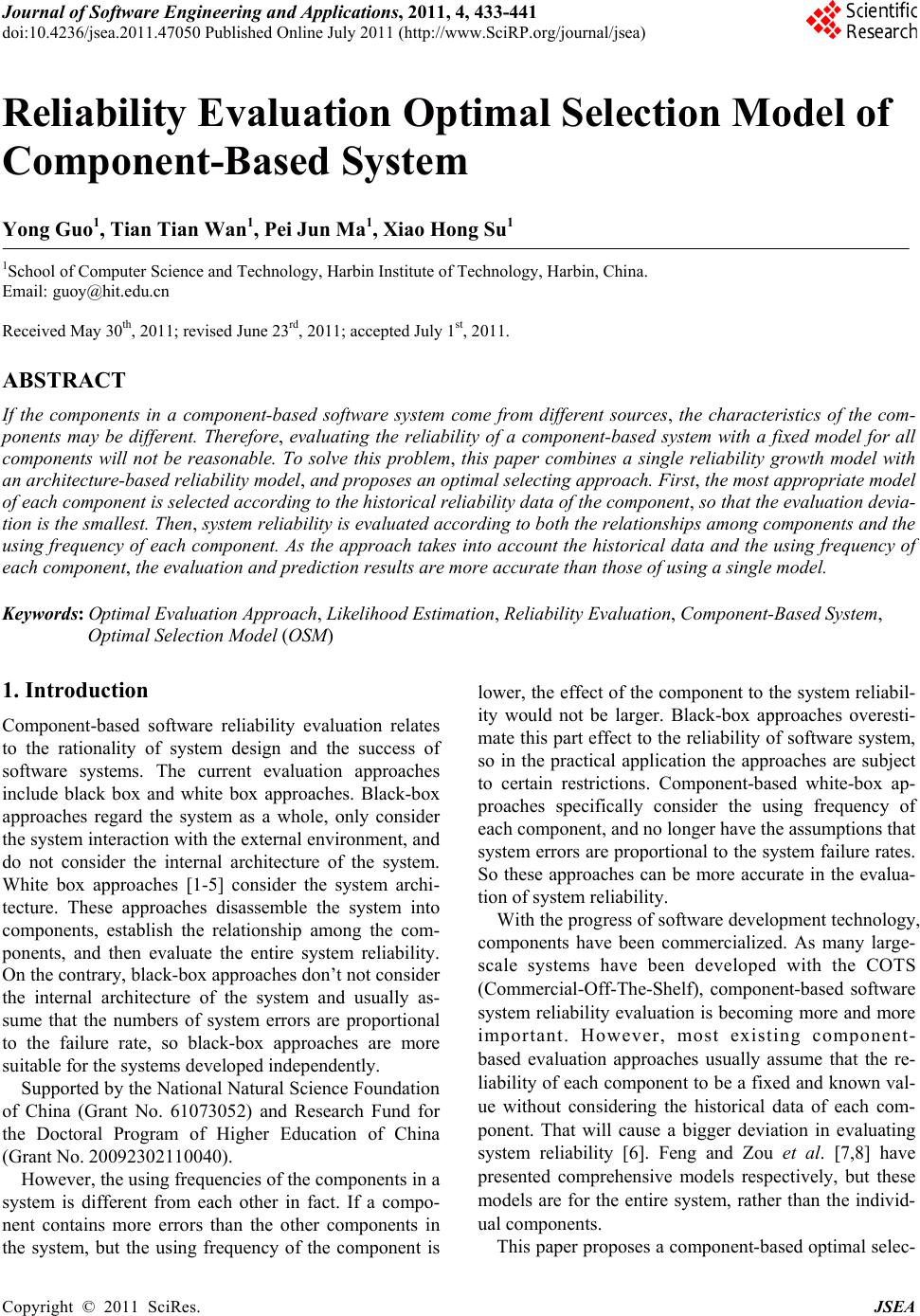
Journal of Software Engineering and Applications, 2011, 4, 433-441
doi:10.4236/jsea.2011.47050 Published Online July 2011 (http://www.SciRP.org/journal/jsea)
433
Reliability Evaluation Optimal Selection Model of
Component-Based System
Yong Guo1, Tian Tian Wan1, Pei Jun Ma1, Xiao Hong Su1
1School of Computer Science and Technology, Harbin Institute of Technology, Harbin, China.
Received May 30th, 2011; revised June 23rd, 2011; accepted July 1st, 2011.
ABSTRACT
If the components in a component-based software system come from different sources, the characteristics of the com-
ponents may be different. Therefore, evaluating the reliability of a component-based system with a fixed model for all
components will not be reasonable. To solve this problem, this paper combines a single reliability growth model with
an architecture-based reliability model , and proposes an optim al selecting approach. First, the most appropriate model
of each componen t is selected acco rd ing to the histo rica l reliab ility d ata of th e comp onent , so that the evaluation devia-
tion is the smallest. Then , system reliability is evaluated according to both the relationships among compon ents and the
using frequency of each component. As the approach takes into account the historical data and the using frequency of
each component, the evaluation and prediction results ar e more accurate than those of using a single model.
Keywords: Optimal Evaluation Approach, Likelihood Estimation, Reliability Evalua tion, Component-Based System,
Optimal Sel ect i on Model (OSM)
1. Introduction
Component-based software reliability evaluation relates
to the rationality of system design and the success of
software systems. The current evaluation approaches
include black box and white box approaches. Black-box
approaches regard the system as a whole, only consider
the system interaction with the external environment, and
do not consider the internal architecture of the system.
White box approaches [1-5] consider the system archi-
tecture. These approaches disassemble the system into
components, establish the relationship among the com-
ponents, and then evaluate the entire system reliability.
On the contrary, black-box approaches don’t not consider
the internal architecture of the system and usually as-
sume that the numbers of system errors are proportional
to the failure rate, so black-box approaches are more
suitable for the systems developed independently.
Supported by the National Natural Science Foundation
of China (Grant No. 61073052) and Research Fund for
the Doctoral Program of Higher Education of China
(Grant No. 20092302110040).
However, the using frequencies of the components in a
system is different from each other in fact. If a compo-
nent contains more errors than the other components in
the system, but the using frequency of the component is
lower, the effect of the component to the system reliabil-
ity would not be larger. Black-box approaches overesti-
mate this part effect to the reliability of software system,
so in the practical application the approaches are subject
to certain restrictions. Component-based white-box ap-
proaches specifically consider the using frequency of
each component, and no longer have the assumptions that
system errors are proportional to the system failure rates.
So these approaches can be more accurate in the evalua-
tion of system reliability.
With the progress of software development technology,
components have been commercialized. As many large-
scale systems have been developed with the COTS
(Commercial-Off-The-Shelf), component-based software
system reliability evaluation is becoming more and more
important. However, most existing component-
based evaluation approaches usually assume that the re-
liability of each component to be a fixed and known val-
ue without considering the historical data of each com-
ponent. That will cause a bigger deviation in evaluating
system reliability [6]. Feng and Zou et al. [7,8] have
presented comprehensive models respectively, but these
models are for the entire system, rather than the individ-
ual components.
This paper proposes a component-based optimal selec-

Reliability Evaluation Optimal Selection Model of Component-Based System 434
tion model (OSM). This approach bases on the system
architecture, fully utilizes the historical data of each
component, and takes into account the software reliabil-
ity growth. OSM combines the reliability growth model
of every single component with the architecture-based
reliability model. It selects the proper evaluation model
of component according to the specific characteristic of
each component, and then synthetically evaluates the
system reliability according to the relationships among
these components in the overall system. As the proposed
approach selects the most suitable component evaluation
model according to the characteristics of each component
when evaluating component reliability, the evaluation
result of each component is more accurate. As a result,
the reliability evaluation result of the system is also more
accurate.
The contribution of this paper is that the OSM is pro-
posed. The OSM combines a single reliability growth
model with an architecture-based reliability model. As
the new model takes into account the historical data and
the using frequency of each component, the evaluation
and prediction results are more accurate.
The organization of this paper is organized as follows.
In Section 2, we will give a survey of existing component
reliability models and component-based system reliabil-
ity models. In Section 3, the OSM operation process is
described. In Section 4, approach of selecting component
reliability model is presented. In Section 5, the software
reliability evaluation approach is discussed. In Section 6,
case analysis and verification is demonstrated. Finally,
the conclusion remarks are given in Section 7.
2. Component Reliability Model and
Component-Based System Reliability
Model
A component usually refers to executable modules that
encapsulate data and function. Components can be inde-
pendently produced or developed by the third parties.
Usually these approaches that evaluate the system reli-
ability considering the system as a whole [9-18] can be
used to evaluate a single component. We can select a
proper model according to the component’s historical
data. We can also use a certain model by translating the
component’s historical data into the form that the model
can be used. According to different historical reliability
data that the models can use, the component reliability
models can be divided into two categories, i.e. the time
between failure (TBF) models [9-12] and the failure
count (FC) models [13-18]. TBF models use time-bet-
ween-failure data, while FC models use the failure count
data.
A system constructed by components with logical re-
lation is called component-based system. Component-
based system reliability evaluation models include path-
based approach [1,2,19], state-based approach [3-5,20,
21], and additive model [22]. Path-based approaches [1-2,
19] evaluate system reliability by considering all the pos-
sible execution paths of the software. A sequence of all
execution paths are gained by algorithm, experiment or
simulation. The reliability of each path is estimated, and
then the system reliability is estimated by calculating the
average reliability of all paths. State-based models
[4,5,20,21] regard the execution of the software as a state
transfer process [6]. This class of models apply stochastic
process theorem to the analysis of the system reliability.
Some typical approaches adopt the Markov process the-
ory, which assume that the system change process with
the state of Markov. The approaches include the discrete
time Markov model (DTMC) [5,20] and the time con-
tinuous Markov model (CTMC) [4] and semi-Markov
process (SMP) [21]. Additive models [22] are mainly
used in the software testing stage. It assumes that the
reliability of each component can be modeled by non-
homogeneous Poisson process (NHPP), and thus the
failure behavior of the system will also be a NHPP [23].
Path-based and state-based models typically assume
that the reliability of components is known, and no long-
er consider the problem of the reliability evaluation for
each component. Additive models concentrate on system
failure-sensitive issues of time concerned by evaluating
the component failure, but no longer explicitly consider
the system architecture. To establish an effective com-
ponent-based reliability evaluation model, we should
take into account the evaluation approach of each com-
ponent in a system. Only by doing this, can we get a
more reasonable evaluation result.
3. OSM Operation Process
This paper gives the following relevant definitions as a
basis of OSM.
Definition 1 Failure interval time data(TBF). It is a tri-
ple<F,T,S>, where F is one-dimensional vector repre-
senting the failure order, T is the one-dimensional vector
representing interval between the two adjacent failure, S
is the one-dimensional vector representing the severity of
the failure. For any element f in F, there is only one ele-
ment tf in T, and sf in S to correspond to it, which
<f,tf,sf> constitutes a TBF data.
Definition 2 Failure count data FC. It is a four tuple <I,
T0,C, S>, where I is one-dimensional vector representing
the test number, T0 is the time interval, C is one-dimen-
sional vector composed of errors during the interval T0, S
is one-dimensional vector composed of the severity of
the error during the interval T0. <i,T0,ci,si> is a failure
count data, where i is an element in I, ci is an element in
C, si is an element in S.

Reliability Evaluation Optimal Selection Model of Component-Based System435
Definition 3 Components. It is a four tuple <F,P,D,M>,
where F is a group of service interface to the outside
provided by the component, P is the description of the
component external behavioral, D is the reliability of the
application domain, M is the reliability-related data of the
component.
Definition 4 TBF component. It is a class of compo-
nent that its reliability-related data is of the type TBF.
Definition 5 FC component. It is a class of component
that its reliability-related data is of the type FC.
The OSM operation process of a component-based
system is shown in Figure 1.
The first step of OSM is that all the components of the
system are determined. These components are obtained
from the requirements analysis and design documents, and
then assorted. The types of reliability-related historical
data may be different, because the components come from
different sources, and their specific implementation tech-
niques, methods and testing process may be different. The
components are divided into two categories: TBF compo-
nents and FC components, mainly based on the type of the
components’ historical data. Then, the candidate reliability
model sets of the component are determined.
According to the categories of components and the ap-
plication scope of the selected model, we determine the
candidate reliability model sets of the component. For
TBF components, all models in the candidate model set
should belong to the class of TBF. For FC components,
all models in the candidate model set should belong to be
the class of FC. As each component is considered as a
Figure 1. The OSM process of component-based system
reliability evaluation approach.
whole and its internal structure is no longer considered,
black-box evaluation approaches are used. According to
the software life-cycle, the classes of software reliability
models include the analysis phase model, the design
phase model, the implementation phase model, the test-
ing phase model and the validation phase model. For the
purpose of reliability evaluation of component-based
software systems, the test phase model for each compo-
nent is used to determine the component’s reliability in
OSM.
After that, the evaluation criteria are applied. At pre-
sent there is not any universal component reliability
model, which means no model can be suitable for the
reliability evaluation of all kinds of components. In order
to evaluate the reliability of each component more effec-
tively, evaluation criteria are used. There are many types
of evaluation criteria. We can adopt a single criterion or a
combination of several evaluation criteria. The single
evaluation criterion means that the final component
evaluation model is determined by a single formula. The
combination evaluation approach is a combination of
multiple evaluation criteria, such as the statically
weighted combination. According the computing result
of every component by the combination approach, the
evaluation model of every component is determined. The
complexity and practicality of the algorithm should be
taken into account in determining the criteria. If the
evaluation approach is too complicated, its practicality
will be reduced. It is not that the more complex the selec-
tion method is, the better it is. The details of the evalua-
tion criteria and selection methods will be given in part 5.
Next, the evaluation model and the prediction model
are obtained. We should consider from the two sides of
evaluation model and prediction model when we select
the component reliability model, because our ultimate
goal is to obtain system reliability. System reliability
evaluations include the assessment and prediction. Sys-
tem reliability assessment usually refers to the reliability
the system can be achieved when the development of the
software system is completed, and the system reliability
prediction is to predict the system failure at a future point
when the system is running. So the system reliability
evaluation includes the assessment and the prediction.
The optimal model for assessment is not necessary the
optimal model for prediction, so the assessment model
and prediction model should be selected respectively.
Finally, based on the prediction and assessment model,
the system reliability is obtained according to the rela-
tionship among the components.
4. Approach of Selecting Component
Reliability Model
In order to accurately assess and predict the reliability of

Reliability Evaluation Optimal Selection Model of Component-Based System 436
each component, we should use appropriate method and
criteria to select the most suitable model of the compo-
nent reliability.
4.1. Principle of Selecting Approach
Let

12
, ,,
n

M
MM M be a set that contains n
candidate reliability model sets. Every model seti
M
in M
contains i models, i
. Different
types of models suit for different data sets. Assuming the
type of i
N

12
, ,,
iN
Mmm m
M
model suits for the historical data sets Di,
the evaluation criterion corresponding to i
M
is i, i
is the result calculated by the combination of weight
indexes, t
S
kS
s
is the t-th indicators in , t is the
weight corresponding to st. We have the following Equa-
tion (
k w
1).
1
k
i
t
Ss

t
t
w (1)
Let C is the components set in which its system reli-
ability will be evaluated. 12
{, ,,}
m
Ccc c


c
，there are
m components, where component t can use the type of
i
M
model to compute its reliability. Which type of
model specifically will be used depends upon the reli-
ability data of component. tj corresponds to the com-
ponent t of set C and model mi of Mi. The value of
tj is computed using Equation (
S
m
t
c
optim{, ,,
ttt
c
S1). If t is the opti-
mal evaluation model of component , the value st sat-
isfies the conditions: 11 1t }
s
SSS,“optim”
is min or max according to the specific indicators. The
candidate model and selection criteria will be described
specifically later.
4.2. Component Candidate Evaluation Model
There are many factors affecting software reliability. The
affect of the same factor is different to different software.
Many factors have the stochastic characteristic time-
related, so the software reliability models are mostly
modeled the form of random process. A number of as-
sumptions are given in advance for the establishment of
models. Under the assumption we establish systems reli-
ability evaluation model.
 FC models
1) Schick-Wolverton model [9]
The state when the software is tested is same as its ac-
tual operation. All errors have the same probability to be
detected. The expectations of failure occur at any interval
are proportional to the number of errors contained in the
software and the duration after the last occurrence of
failure. All failures have the same severity and inde-
pendently one another. Faults are corrected as soon as
they are found and there is no new fault to be introduced.
[24]
2) Non-Homogeneous Poisson for FC [10]
The state when the software is tested is same as its ac-
tual operation. The number of faults detected in each
time is independent one another. All faults have the same
probabilities to be detected. The total number of faults
detected in any time fallows a Poisson distribution with
mean m(t). The mean value of faults is a bounded
non-decreasing function related to m(t) and its max value
is a. There is no new fault to be introduced when the de-
tected faults are corrected. [24]
3) Schneidewind [11]
The state when the software is tested is same as its ac-
tual operation. The system failure caused by faults is
stochastic. The occurrences of all failures have the same
probability and independent of one another. The correc-
tion rate of fault is proportional to the found faults. The
detected failures mean value decrease with the continu-
ous test. The total number of failures has an upper bound.
Every test has the same period interval. The faults detec-
tion rate is proportional to the number of system faults.
There is no new fault to be introduced when the detected
faults are corrected. [24]
4) Yamada S-shaped model [12]
The state when the software is tested is same as its ac-
tual operation. The system failure caused by faults is
stochastic. The number of initial faults in the software
system is a random variable. The time between failures
(k – 1) and k depends on the time to failure (k – 1). Only
one failure occurs each time and the fault will be cor-
rected immediately. There is no new faults are introduced
when the detected fault is removed. The total number of
failures has an upper bound. [24]
 TBF models
1) Geometric model [13]
The test process is same as its actual operation. There
is no upper bound on the total number of failures. The
probability of all faults detection is equal. The detections
of all faults are independent each another. The failure
detection rate is geometric distribution and is constant
between failure occurrences. [24]
2) Jelinski-Moranda model [14]
The condition of the software run is same as its actual
operation. The faults detection rate is proportional to the
number of the faults. The severity of all failures is equal.
The failure rate between the two failures is a constant
value. Faults are removed immediately and no new fault
is introduced. The total number of faults has an up bound.
[24]
3) Littlewood-Verrall model [15]
The condition of the software run is same as its actual
operation. The successive time between two failures is
independent random variable and is an exponential dis-
tribution. The mean of i-th failure distribution is 1/  (i),
 (i) has  distribution with parameter  and  (i). Where
 (i) has the form  (0)+  (1) * i or  (0)+  (1) * i2. There is

Reliability Evaluation Optimal Selection Model of Component-Based System 437
no upper bound on the total number of failures. [24]
4) Musa Basic model [16]
The test process is same as its actual operation. The
detection of faults is independent one another. All faults
of the system will be detected. The intervals between the
successive failure are piecewise exponential distribution.
The failure rate is proportional to the number of faults.
The correction rate is proportional the fault detection rate.
There is no new fault to be introduced when the fault is
corrected. [24]
5) Musa-Okumoto model [17]
The test process is same as its actual operation. The
detection of faults is independent one another. The mean
of the number of failures is a logarithmic function of
time. The intensity of failure decreases exponentially
with the experience of failures. The total of faults has an
up bound. [24]
6) Non-Homogeneous Poisson Process model [18]
The condition of the software run is same as its actual
operation. All faults have the same probability to be ob-
served. The cumulative number of failure M(t) follows a
Poisson distribution with mean value m(t). The mean
function of the number of failure is a bounded non-de-
creasing. The debug process will not introduce new fail-
ure. [24]
The models mentioned-above are subject to assump-
tions, therefore there are some limitations, no model can
replace another.
4.3. Determination of the Selection Criteria
The effect is different when one model is applied on dif-
ferent data sets, one may be good but others may be bad.
We can select the most suitable evaluation model ac-
cording to a certain criterion using a certain data set. The
key is the determination of the criterion when we select
the suitable model. The commonly criteria are deviation
of Bias, mean square error MSE, mean absolute error
MAE, MSE and sum squire error SSE , chi-square test
(Chi-Square), CKolmogorov-Smirnov test) prequential
likelihood(PL) .
Chi-square test is a common method that measures
model goodness of fit. The smaller result means a better
goodness of fit, The formula is shown as (2).




2
1
nii
ii
mmt
CHS mt




 (2)
The Kolmogorov-Smirnov test (K-S test) is a test of
goodness of fit. It is used to study if the distribution of
sample observations agrees with the specified theoretical
distribution. The two-sample K-S test is one of the most
useful and general nonparametric methods for comparing
two samples, as it is sensitive to differences in both loca-
tion and shape of the empirical cumulative distribution
functions of the two samples. The K-S statistic quantifies
a distance between the empirical distribution function of
the sample and the cumulative distribution function of
the reference distribution, or between the empirical dis-
tribution functions of two samples. The formula is (3),
where F(x) and E(x) are the theoretical and actual distri-
bution of the sample respectively.
  
max maxDFxE

x (3)
The formulas mentioned above are mainly used to se-
lect component assessment model. As to the selection of
reliability predictive model of component, we often use
prequential likelihood. Prequential likelihood values are
used to indicate if one model is more applicable to the
failure data than the other models. Let
j
t is the next
time of component failure, the failure distribution density
function estimated by previous failure data is
1
j
t


j
j
f
t

, according to the density function we can esti-
mate the next system failure time tj, the expectation of tj
is:

0
ˆd
jj
Etf tt

 
  (4)
For the 1-step prediction, the prequential likelihood
value for 12
,,,
j
j
tt t
jn



i
is calculated as (5).

nj
ni
ijl
PLf t




(5)
This paper will use K-S test and Chi-square test as the
selection criteria of reliability assessment model of
component. They are commonly used in project. This
paper will use prequential likelihood value as the selec-
tion criterion of reliability predictive model of compo-
nent.
4.4. System Reliability Calculation
According to the Relationship among
Components
We will determine the interaction among the components
of the system after the determination of the evaluation
and prediction models of the component. We can model
path-based system component diagram, state-based sys-
tem components diagrams or other system component
interaction diagram. It will depend on the actual specific
situation. If the software continuously runs 24 h every
day, it should be modeled as Continuous Time Markov
Chains (CTMCs). If it is operated by user’s idea, it
should be modeled as Discrete Time Markov Chains
(DTMCs). At the same time we should also consider the
available data, the different phase of the software
life-cycle and what kink of assumptions we made [25].
Table 1 lists the state-based Markov models and appli-
cable conditions [25].

Reliability Evaluation Optimal Selection Model of Component-Based System 438
Table 1. Reliability models.
Architectural ModelSolution MethodReliability
DTMC_1 absorbing Composite


1, n
R
SnR
DTMC_2 absorbing Hierarchical
1
i
V
i
i
n
R
R



DTMC_3 absorbing Hierarchical
1
eiii
nVt
i
R
 


DTMC_4 absorbing Hierarchical 0()d
1
e
Vt
ii i
n
i
R

 



DTMC_5 irreducible Composite
DTMC_6 irreducible Hierarchical
1
n
ii
i
R
R




DTMC_7 irreducible Hierarchical
1
n
ii
i






,e
t
R



CTMC_1 absorbing Composite
CTMC_2 absorbing Hierarchical ()
1
eii
n
L
t
i
R
 


CTMC_3 absorbing Hierarchical
1
i
nV
i
i
R
R



CTMC_4 absorbing Hierarchical
()
0()d
1
e
Lt
ii
n
i
R

 



CTMC_5 irreducible Composite
CTMC_6 irreducible Hierarchical
1
n
ii
i






,et
R



CTMC_7 irreducible Hierarchical
1
n
ii
i
R
R




As the space limited, please refer to related literature
about how to establish relationship among the compo-
nents of system. After the system model established, the
system reliability can be predicted and assessed. As the
assessment and prediction reliability value of each com-
ponent are optimal according to the criteria, and therefore
the assessment and prediction reliability of the system
will also be optimal. We will prove this point as follows.
5. Discussion of Software Reliability
Evaluation Approach
Let system composed by n components, the reliability of
components computed by OSA are 12 , the
exact value of the components reliability are
12 respectively. The system reliability calcu-
lated by a certain model using the exact value of each
component reliability 12 is . The
system reliability calculated by the model using the
evaluation value of each component reliability
12 n is
,,,
n
RR R 

=i RfR
,,,
n
RR R
,,,RR
,,,
n
RR R

R

i
RfR . is the difference
between and
R
R R



'Rii fR fR RR
If the smaller i
R


,
n
R
is the smaller is, then we can
say the system reliability calculated using the component
models selected by OSA is more accurate than other
component models. It is not difficult to see from Table 1
that the system reliability models listed in Table 1 is
consistent with the hypothesis mentioned above. We will
use CTMC_7 as a sample to demonstrate this point. The
formula of model CTMC_7 is showed as (
R
R
,,
7).
1
n
ii
i
R


 (6)
Let is the system reliability calculated by exact
value 12 using formula (
0
R
RR ,, 6), is the sys-
tem reliability calculated by 12 using for-
mula (
0
R
,
n
RRR
6). The difference between R and R′ is:

11
iii i
R RRR


nn
i
ii
RR  

(7)


From (7) we can see the smaller the error i R

 of
each component is, the smaller the error of the sys-
tem.
R

Reliability Evaluation Optimal Selection Model of Component-Based System439
As the models of components are selected using OSA,
there is

_
122
min, , ,,
selectd model
model modelmodelmodeln
R
RRR R

 
so that we can get more accurate system reliability by the
approach proposed in this paper.
6. Case Analysis and Verification
We use following system shown in Figure 2 as an exam-
ple. The system is composed by the three components.
We use state-based reliability model to model it. In order
to facilitate to model it, we add a termination state E, a
completion state C, and a failure state F, the starting
component is C1. The historical data of components C1,
C2, C3 are provided by CASRE20, the specific values
shown in Table 2. The historical data of component C1,
C2 are time between failures data, the historical data of
component C3 is the failure count data. Because different
types of component model is suit for different reliability
Figure 2. Components relationship of the system.
data, we should use TBF model for component C1 and
C2 , FC model for component C3.
Table 2 shows these components historical reliability
data.
According to the approach presented in 5.1 and the
criteria in 5.2, the results are shown as Table 3.
From the results in Table 3 we can see the best good-
ness of fit reliability assessment models of components
C1, C2, C3 are Quadratic LV (KS Distance = 10.67302),
Quadratic LV(KS Distance = 14.68409) and Schick-
Table 2. The historical reliability data of component C1, C2, C3.
C1 C2 C3
No. Duration Since Last Failure severity No.Dura t i o n S i nce Last Failureseverity No.Failure count Interval severity
1 3 1 139 1 114 56.0 1
2 30 1 210 1 219 56.0 1
3 113 1 34 1 323 56.0 1
4 81 1 436 1 412 56.0 1
5 115 1 54 1 522 56.0 1
6 9 1 65 1 612 56.0 1
7 2 1 74 1 713 56.0 1
8 91 1 891 1 819 56.0 1
9 112 1 9 49 1 910 56.0 1
10 15 1 101 1 105 56.0 1
11 138 1 1125 1 115 56.0 1
12 50 1 121 1 125 56.0 1
13 77 1 134 1 137 56.0 1
14 24 1 1430 1 147 56.0 1
15 108 1 1542 1 151 56.0 1
16 88 1 169 1 163 56.0 1
17 670 1 1749 1 171 56.0 1
18 120 1 1844 1 182 56.0 1
19 26 1 1932 1 190 56.0 1
20 114 1 203 1 202 56.0 1
21 325 1 2178 1 219 56.0 1
22 55 1 221 1 221 56.0 1
23 242 1 2330 1 230 56.0 1
24 68 1 24205 1 240 56.0 1
25 422 1 255 1 250 56.0 1
26 180 1 26129 1 261 56.0 1
27 10 1 27103 1 271 56.0 1
28 1146 1 28224 1
29 600 1 29186 1
30 15 1 3053 1

Reliability Evaluation Optimal Selection Model of Component-Based System 440
Table 3. The results of components candidate models.
C1 C2 C3 Components
Candidate Models –1 * ln(PL) KS Distance–1 * ln(PL)KS Distance
Components
Candidate Models –1 * ln(PL) Chi-Square
Geometric Model 29.2264 10.688 24.6318 14.72469 Generalized Posson 30.5155 26.53031
Jelinski-Moranda 30.3014 901.7729 24.6462 16.53530 Yamada S-Shaped 33.4908 33.54718
Linear LV 29.6216 11.02811 25.8762 17.42809 Schneidewind 30.8320 34.17516
Musa Basic 29.7884 900.4869 24.7259 16.23364 Schick-Wolverton 30.5155 26.53030
Musa-Okumoto 29.2700 898.9216 24.7884 16.02850
NHPP 29.7884 900.4869 24.7259 16.23364
Quadratic LV 29.0415 10.67302 24.8086 14.68409
Table 4. The selected models of each component and the system reliability.
assessment
prediction(T = 50) i

selected models Ri selected models Ri
C1 Quadratic LV 0.9977
Jelinski-Moranda 0.93640 0.2350
C2 Quadratic LV 0.9903
Linear LV 0.53740 0.5199
C3 Schick-Wolverton 0.9999 Yamada S-Shaped 0.99993 0.2451
Rs 0.9944 0.7445
Wolverton (Chi-Square = 26.53030) respectively. The
best goodness of fit reliability prediction models of
components C1, C2, C3 are Jelinski-Moranda(–1 * ln(PL)
= 30.3014), Linear LV(–1 * ln(PL) = 25.8762) Yamada
S-Shaped(–1 * ln(PL) = 33.4908) respectively. Assuming
system reliability evaluation use DTMC_6 and i

is
known. The assessment and prediction values are shown
in Table 4. The assessment value refers to the reliability
when the system development is completed, the predic-
tion value refers to the system reliability at a certain time
T in the future. Here we set T to be 50. T can be changed
to predict the system reliability at other time point.
7. Conclusions
An optimal selection approach to improve the evaluation
accuracy of component-based system reliability is pro-
posed in this paper. The techniques of how to select the
most appropriate assessment and prediction model for
each component according to historical data based on
certain criteria, and how to assess and predict the system
reliability according to the selected model and the rela-
tionships among the various components, are presented.
This approach considers not only the architecture of the
system but also the historical data related to each com-
ponent reliability growth. As a result, its results are more
effective and practical than those of the other existing
approaches.
REFERENCES
[1] H. Singh, et al., “A Bayesian Approach to Reliability
Prediction and Assessment of Component Based Systems,”
Proceedings of 12th International Symposium on Software
Reliability Engineering, Hong Kong, 27-30 November
2001, pp. 12-21.
[2] S. Yacoub, et al., “A Scenario-Based Reliability Analysis
Approach for Component-Based Software,” IEEE Trans-
actions on Reliability, Vol. 53, No. 4, 2004, pp. 465-480.
doi:10.1109/TR.2004.838034
[3] B. Littlewood, “Software Reliability Model for Modular
Program Structure,” IEEE Transactions on Reliability,
Vol. R-28, No. 3, 1979, pp. 241-246.
doi:10.1109/TR.1979.5220576
[4] S. S. Gokhale and L. Michael Rung-Tsong, “A simulation
Approach to Structure-Based Software Reliability Ana-
lysis,” IEEE Transactions on Software Engineering, Vol.
31, No. 8, 2005, pp. 643-656. doi:10.1109/TSE.2005.86
[5] Y. Wei and X.-H. Shen, “Heterogeneous Architecture-
-Based Software Reliability Estimation: Case Study,” 3rd
International Conference on Convergence and Hybrid
Information Technology, Busan, 11-13 November 2008,
pp. 286-290.
[6] S. S. Gokhale, “Architecture-Based Software Reliability
Analysis: Overview and Limitations,” IEEE Transactions
on Dependable and Secure Computing, Vol. 4, No. 1,
2007, pp. 32-40. doi:10.1109/TDSC.2007.4
[7] Z. F. Zhong and X. R. Zuo, “Multi-model Assessment of
Software Reliability,” Journal of TongJi University, Vol.
30, No. 10, 2002, pp. 1183-1185.
[8] F. G. Cheng, et al., “Software Reliability Growth Model
Selection and Composition Method,” Computer Science,
Vol. 36, No. 9, 2009, pp. 135-138.
[9] R. W. W. G. J. Schick, “Assessment of Software Relia-
bility,” Operations Research, Physica-Verlag, Heidelberg,
1973, pp. 395-422.
[10] H. Chin-Yu, et al., “A Unified Scheme of Some Non-
homogenous Poisson Process Models for Software Relia-
bility Estimation,” IEEE Transactions on Software Engi-
neering, Vol. 29, No. 3, 2003, pp. 261-269.
doi:10.1109/TSE.2003.1183936
[11] N. F. Schneidewind, “Analysis of Error Processes in

Reliability Evaluation Optimal Selection Model of Component-Based System441
Computer Software,” Proceedings of the International
Conference on Reliable Software, Los Angeles, 21-23
April 1975, pp. 337-346. doi:10.1145/800027.808456
[12] S. Yamada, et al., “S-Shaped Reliability Growth Mode-
ling for Software Error Detection,” IEEE Transactions on
Reliability, Vol. R-32, No. 5, 1983, pp. 475-484.
doi:10.1109/TR.1983.5221735
[13] P. B. Moranda, “An Error Detection Model for Appli-
cation during Software Development,” IEEE Transac-
tions on Reliability, Vol. R-30, No. 4, 1981, pp. 309-312.
doi:10.1109/TR.1981.5221096
[14] Z. A. M. Jelinski, “Software Reliability Research,” Aca-
demic Press, New York, 1972.
[15] B. Littlewood, “The Littlewood-Verrall Model for Software
Reliability Compared with Some Rivals,” Jour- nal of
Systems and Software, Vol. 1, 1979, pp. 251-258.
doi:10.1016/0164-1212(79)90025-6
[16] J. D. Musa, “A Theory of Software Reliability and Its
Application,” IEEE Transactions on Software Enginee-
ring, Vol. SE-1, No. 3, 1975, pp. 312-327.
[17] J. D. Musa and K. Okumoto, “A Logarithmic Poisson
Execution Time Model for Software Reliability Mea-
surement,” Proceedings of the 7th International Confe-
rence on Software Engineering, Orlando, 26-29 March
1984, pp. 230-238.
[18] A. L. Goel and K. Okumoto, “Time-Dependent Error-De-
tection Rate Model for Software Reliability and Other
Performance Measures,” IEEE Transactions on Reliability,
Vol. R-28, No. 3, 1979, pp. 206-211.
doi:10.1109/TR.1979.5220566
[19] M. L. Shooman, “Structural Models for Software Reliabi-
lity Prediction,” Proceedings of the 2nd International
Conference on Software Engineering, San Francisco,
13-15 October 1976, pp. 268-280.
[20] R. C. Cheung, “A User-Oriented Software Reliability
Model,” IEEE Transactions on Software Engineering,
Vol. SE-6, No. 2, 1980, pp. 118-125.
doi:10.1109/TSE.1980.234477
[21] P. Kubat, “Assessing Reliability of Modular Software,”
Operations Research Letters, Vol. 8, No. 1, 1989, pp. 35-
41. doi:10.1016/0167-6377(89)90031-X
[22] W. Everett, “Software Component Reliability Analysis,”
1999 IEEE Symposium on Application-Specific Systems
and Software Engineering and Technology, Richardson,
24-27 March 1999, pp. 204-211.
[23] K. Goseva-Popstojanova and K. S. Trivedi, “Architecture-
Based Approaches to Software Reliability Prediction,”
Computers & Mathematics with Applications, Vol. 46, No.
7, 2003, pp. 1023-1036.
doi:10.1016/S0898-1221(03)90116-7
[24] A. P. Nikora, “CASRE User’s Guide,” Jet Propulsion
Laboratories, Pasadena, 2000.
[25] S. S. Gokhale and K. S. Trivedi, “Analytical Models for
Architecture-Based Software Reliability Prediction: A
Unification Framework,” IEEE Transactions on Reliability,
Vol. 55, No. 4, 2006, pp. 578-590.
doi:10.1109/TR.2006.884587