Journal of Software Engineering and Applications, 2011, 4, 426-432
doi:10.4236/jsea.2011.47049 Published Online July 2011 (http://www.SciRP.org/journal/jsea)
Mapping Software Metrics to Module Complexity:
A Pattern Classification Approach
Nick John Pizzi
Department of Computer Science, University of Manitoba, Winnipeg, Canada.
Received June 3rd, 2011; revised June 30th, 2011; accepted July 1st, 2011.
ABSTRACT
A desirable software engineering goal is the prediction of software module complexity (a qualitative concept) using
automatically generated software metrics (quantitative measurements). This goal may be couched in the language of
pattern classification; namely, given a set of metrics (a pattern) for a software module, predict the class (level of com-
plexity) to which the module belongs. To find this mapping from metrics to complexity, we present a classification
strategy, stochastic metric selection, to determine the subset of software metrics that yields the greatest predictive pow-
er with respect to module complexity. We demonstrate the effectiveness of this strategy by empirically evaluating it us-
ing a publicly available dataset of metrics compiled from a medical imaging system and comparing the prediction re-
sults against several classification system benchmarks.
Keywords: Software Metrics, Pattern Classification, Feature Selection, Software Complexity
1. Introduction
Software systems are used to solve or model increas-
ingly complex problems in a variety of application do-
mains. However, problem complexity should not mani-
fest itself as software module complexity. That is, prob-
lem complexity should only produce software complex-
ity as an emergent property and not as an intrinsic prop-
erty of individual software modules (functions, objects,
templates, and so on). Intrinsic module complexity is an
undesirable characteristic that is often subjectively iden-
tified by software developers for some form of remedial
action. However, this subjective process is slow, tedious,
and error-prone. Automating (to some extent) this proc-
ess would be desirable especially if coupled with a more
rigorous quantitative approach. One possible strategy is
the prediction of software module complexity using auto-
matically generated quantitative measurements, namely
software metrics [1,2].
A software metric is a mapping from a software mod-
ule to a set of numerical values to quantify one or more
software attributes [3]. These metrics are commonly re-
garded as important factors reflecting the nature of soft-
ware systems including, among other characteristics, the
property of complexity [4-7]. Software complexity has a
direct influence on its quality, clarity, extensibility, and
maintainability. The analysis of complexity may be cast
as a problem of pattern classification: find a mapping that
predicts the class label (level of software complexity) of
a pattern (software module), given only its features
(software metrics). Such a classification system could
serve as a “complexity filter” for software modules. For
instance, a project manager or software developer could
use such a filter to predict module complexity to identify
highly complex software modules for review and possi-
ble revision.
While some metrics may have discriminatory power,
that is, predictive utility vis-à-vis complexity, other met-
rics may have none. Moreover, it is possible for some
metrics to have a potential deleterious effect on the clas-
sification process [8-11]; these confounding metrics dis-
tort class boundaries in the metric space (for instance,
delineating between high complexity and low complexity
modules), thereby reducing classification performance
(accuracy). Therefore, it is important not only to identify
discriminatory metrics but to also cull confounding ones.
To this end, stochastic metric selection is investigated as
a pattern classification strategy to determine the subset of
software metrics that best predict software module com-
plexity. The strategy, which stochastically examines
subsets of software metrics for their predictive power, is
empirically evaluated using a database of software met-
rics from a large medical image processing system, and

Mapping Software Metrics to Module Complexity: a Pattern Classification Approach427
the strategy’s classification performance is compared
against several classification system benchmarks. Section
2 presents a brief overview of the dataset’s software met-
rics. Section 3 describes the classification strategy for
finding a mapping between software metrics and module
complexity. Details relating to the design of the experi-
ments and the results compared against the benchmarks
are presented in Section 4 and Section 5, respectively,
with concluding remarks in Section 6.
2. Classification & Software Measurements
Couched in classification terms, we are interested in
finding a mapping between patterns (metrics) and class
labels (complexity); formally, X={(xk, ωk), k = 1,2,…,N}
is a set of N patterns, xk∈
Ը
n, with respective class labels,
ωk ∈={1,2,…,c}. X is randomly allocated to a design
subset (often referred to as a training set), XD, comprising
ND patterns, or a validation subset (often referred to as a
test set), XV, comprising NV patterns (ND + NV = N). A
classification system finds a mapping, f: XD  . Sub-
sequently, f is validated using XV, f: XV  . In our spe-
cific case, X is the dataset described in Section 2.1 where
xk is the list of software metrics (see Section 2.2) for
software module k. As defined in Section 2.3, we will use
c = 2 class labels for complexity: low, ω1, and high, ω2.
It is important to note at this point that the choices for
metrics and class labels described below were made for
the sake of expediency; specifically, these were the pa-
rameters that were supplied in the publicly available da-
taset. Class labels, based on change counts (see Section
2.3), are unlikely to be the best delineators of software
module complexity, nor are the supplied metrics neces-
sarily the best predictors of complexity. No claim is
made as to the optimality of these parameters vis-à-vis
complexity prediction, rather we make the simple prag-
matic assertion that they will serve as an experimental
test bed to examine the efficacy of treating the assess-
ment of software module complexity as a problem of
pattern classification.
2.1. Medical Imaging System
This investigation considers the Medical Imaging System
(MIS) dataset [12] that has been used in some other stu-
dies dealing with software quality [13,14]. MIS is a
commercial software system consisting of approximately
4500 modules and comprising approximately 400000
lines of code. The dataset consists of N = 390 software
modules. Each module is described using n = 11 software
metrics as well as its change count, which is a reflection
of its complexity [7].
2.2. Software Metrics
As the software engineering literature provides thorough
and extensive discussions of the software metrics used in
this investigation, including their relative advantages and
disadvantages [13,15-17], we restrict ourselves to brief
summaries. The first software metrics collected for each
MIS module are the ubiquitous “lines of code” (L1),
which is the total number of lines of code including pro-
grammer comments, and the number of lines of code
excluding comments (L2). The next set of software
measures includes the number of code characters (C1),
comments (C2), comment characters (C3), and code
characters (C4), respectively.
Another set of software measures pertain to more
complex computations based on the length of a program:
Halstead’s measure of program length (P1), which is the
sum of the total number of program operators and the
total number of program operands [18]; Halstead’s soft-
ware measure of estimated program length (P2), P2 =
η1logη1 + η2logη2, where η1 and η2 are the total number
of unique program operators and program operands, re-
spectively; and, Jensen’s program length (P3), P3 =
(logη1)! + (logη2)! [16].
The final two software measures concern program
control flow graphs: McCabe’s cyclomatic number (F1),
which is one more than the total number of decision
nodes in the control flow graph [19]; and Belady’s
bandwidth metric (F2), F2 = a–1 i (i  ai), where ai is the
number of nodes at level i in a nested control flow graph
of a nodes.
2.3. Change Count
In this investigation, the change count (CC) measure is
used as the class label. While the MIS dataset has 42
unique CC labels, it is unrealistic to expect reliable classi-
fication results using so many class labels with only 390
modules. As a result, the CC class labels are aggregated
into two qualitative classes, low (ω1) complexity versus
high (ω2) complexity, using two different points of de-
lineation, DS3 (no more than three programmer changes)
and DS4 (no more than four programmer changes). The
delineations were arbitrarily chosen, before the classifica-
tion experiments were conducted, so that the two com-
plexity classes were well distributed (roughly an equal
number of software modules in each class).
With DS3, the number of software modules in the low
complexity class is N11 = 192 and the number of software
modules in the high class is N12 = 198, respectively. With
DS4, the number of software modules in the low class is
N21 = 220 and the number of modules in the high class is
N22 = 170.
3. Classification Method
3.1. Stochastic Metric Selection
The motivation for pre-processing strategies exploiting

Mapping Software Metrics to Module Complexity: a Pattern Classification Approach 428
pattern feature selection [20-22] is to simplify the deter-
mination and construction of optimal class boundaries in
the feature space. An example of such a strategy is sto-
chastic metric selection (SMS), which is based on previ-
ous work described in [11] but modified to deal with
software metrics. Figure 1 presents a flowchart of the
iterative SMS algorithm, which individual steps we now
describe below.
The investigator must select the classifier types to be
used; SMS operates with homogeneous or heterogeneous
collections of pattern classifiers e.g., linear discriminant
analysis, artificial neural networks, genetic algorithms,
and support vector machines). The algorithm terminates
upon exceeding a maximum number of iterations, τ, or a
performance (classification accuracy) threshold, PS. A
number of different performance measures may be used
(see Section 4.2). The subsets of metrics are constrained
by four parameters: the minimum and maximum number
of metric subsets, and the minimum and maximum car-
dinality for a metric subset. Metric subsets may also be
quadratically combined to produce “new” metrics (see
below). Using b-fold validation, X is randomly allocated
to either XD or XV. During the design phase, an instantia-
tion of one of the pattern classifier types is used with
randomly sampled metric subsets (satisfying the con-
straints above) from XD to design a mapping. Subse-
quently, during the validation phase, the classification
performance (accuracy), P, is measured using XV. This
process iterates with many pairs of classifier instances
and metric subsets.
SMS exploits the quadratic combination of metric
subsets. The intent is that if the original metric space had
non-linear class boundaries, the new (quadratic) parame-
ter space may end up having class boundaries that are
more linear. SMS has three categories of quadratic com-
binations: using the original metric subset; squaring the
SMS algorithm
(1) Select parameter values, classifiers types, and P.
(2) Repeat while iteration count   and P'  PS:
i) Select metric subsets using histogram.
ii) Perform quadratic transformation of subsets.
iii) Instantiate a classifier type.
iv) Repeat b times (b-fold validation):
a) Randomly allocate X to XD and XV.
b) Design mapping using classifier and XD.
c) Assess performance using XV.
v) If P'  PH, update frequency histogram.
vi) If P' exceeds current best performance, update.
(3) Report best P' (with standard deviation).
Figure 1. Flowchart for SMS algorithm (P' is the median
performance result of a set of b runs).
metric values for a particular metric subset; and using all
pair-wise cross products of metrics from two subsets.
The probabilities (set by the investigator) of selecting
one of these quadratic metric combination categories
must sum to 1.
The stochastic nature of SMS is controlled by a metric
frequency histogram whereby the performance of each
classification task is assessed using the selected per-
formance measure. If the performance exceeds the histo-
gram fitness threshold, PH, the histogram is incremented
at those metric indices corresponding to the subsets used
by the classification task. This metric histogram is used
to generate an ad hoc cumulative distribution function,
which is used when randomly sampling new metric sub-
sets. So, rather than each metric having an equal likeli-
hood of being selected for a new classification task (a
new classifier instance), those software metrics that were
used in previous “successful” classification tasks have a
greater likelihood of being chosen. A temperature term, 0
 t  1, provides additional control over this metric sam-
pling process. If t = 0, the cumulative distribution func-
tion is used but, as t  1, the randomness becomes more
uniform (when t = 1 a strict uniform distribution is used).
3.2. Underlying Classifier
As previously mentioned, the SMS algorithm can operate
with any kind of underlying pattern classifier. In this
investigation, we chose a simple linear pattern classifier
using linear discriminant analysis (LDA) [8], which de-
termines linear class boundaries between c classes (in our
case, complexity) while simultaneously taking into ac-
count between-class and within-class variances. If the
error distributions for each class are the same, it can be
shown that LDA finds the optimal set of linear class
boundaries. In real-world pattern classification situations,
this optimality is seldom achieved since different classes
of patterns typically give rise to different (sometimes,
significantly different) distributions.
The LDA algorithm allocates a pattern, x, to class k for
which the probability distribution, pk(x), is greatest, that
is, x is allocated to class k, if qk pk(x)  qi pi(x) (i  k),
where qk are the prior (or proportional) probabilities. Lk(x)
= logqk + mk
T W–1(x–½mk) is the discriminant function for
class k where mk is the mean for class k and W is the co-
variance matrix. The metric space hyperplane, Fki(x),
separating class k from class i is defined as Fki(x) = Lk(x)
– Li(x) = 0.
4. Experiment Design
4.1. Benchmarks
To assess the effectiveness of SMS for the prediction of
module complexity, we compare it against the perform-

Mapping Software Metrics to Module Complexity: a Pattern Classification Approach429
ance of two classification system benchmarks, the sup-
port vector machine and the radial basis function net-
work.
4.1.1. Support Vector Machine
The support vector machine (SVM) [23,24] is an impor-
tant family of supervised learning algorithms that select
models that maximize the error margin of a training (de-
sign) subset. This approach has been successively used in
a wide range of pattern classification problems [25,26].
Given a set of patterns that are assigned to one of either
two classes, an SVM finds the hyperplane leaving the
largest possible fraction of patterns of the same class on
the same side while maximizing the distance of either
class from the hyperplane. The SVM approach is usually
formulated as a constrained optimization problem and
solved using constrained quadratic programming.
While the original SVM approach [26] could only be
used for linearly separable problems, it may be extended
by employing a “kernel trick” [27] that exploits the fact
that a non-linear mapping of sufficiently high dimension
can project the patterns to a new parameter space in
which classes can be separated by a hyperplane. In gen-
eral, it cannot be determined a priori which kernel will
produce good classification results for a given dataset so
one must rely on heuristic (trial and error) experiments.
Common kernel functions, K(x, y), for patterns, x, y, in-
clude (x × y)d, (ax × y + b)d, tanh(ax × y + b), and
exp(–½|x – y|2/σ).
4.1.2. Radial Basis Function Network
A radial basis function network (RBF) [28], which may
be used for pattern classification, has an internal repre-
sentation of nodes that possess radial symmetry f(x) =
φ(||x–μ||) where: μ is its centre; ||·|| is a distance metric
that determines how far an input pattern is from μ; and,
the transfer function, φ, must output high values when
the distance from a pattern to μ is small, and low values
otherwise. While RBF train quickly [29], selecting the
number of receptive fields is strictly ad hoc. If μi is a
column vector representing the centre of pattern layer
node i and σi is its receptive region diameter, then zi(x) =
exp[–(x – μi)T(x – μi)/(2σi
2) is the output for a given pat-
tern, x. The values μ and σ may analogously be viewed
as the mean and standard deviation of the response curve,
respectively.
The response function of an RBF node diminishes ra-
pidly as patterns deviate from its mean. Here, the pattern
layer weights are trained as well as the location and
shape of the response curves. Standard k-means cluster-
ing is used to compute a μ set. The radius of the normal-
ized zi is determined by σi. If μi is widely separated then
σi should be large to cover the gaps. If they are tightly
packed then σi should be small enough to accurately re-
tain the distinctiveness of each receptive field. P-nearest
neighbor is a standard heuristic algorithm used to deter-
mine σi is. Given a receptive region’s centre, σi, let
i1,…,ip be the indices of the P centres nearest to μi. Then
σi = (P–1p||μi – μip||2)½ (here, P=1).
4.2. Measuring Performance
Selecting a method for measuring the performance (ac-
curacy) of a classification system is often taken for
granted, which often leads to overly optimistic classifica-
tion performance results. Given an n×n confusion matrix
of desired versus predicted class labels, classification
performance is typically measured using the observed
agreement, Po = N–1i nii (i=1,2,…,c), which is the ratio
of patterns that lie in regions associated with their corre-
sponding classes to the total number of patterns regard-
less of where they lie (nii are the diagonal elements of the
confusion matrix). While often used to measure classifi-
cation performance, Po does not take into account the
classification agreement that might be due to chance, Pr =
N–2i (j nij j nji) (i, j=1 ,2 ,…,c) [30]. A more conserva-
tive classification performance measure is the κ score
[31,32], a chance-corrected measure of agreement be-
tween the desired and predicted class assignments, κ =
(Po – Pr)/(1 – Pr). If the classification agreement is due
strictly to chance, κ = 0. If the agreement is greater than
chance κ>0; κ = 1 indicates complete (perfect) agreement.
If the agreement is less than chance then κ < 0 (the min-
imum value depends upon the marginal distributions).
4.3. Parameter Settings
The following parameter values were used with the SMS
algorithm: underlying classifier, LDA; frequency histo-
gram threshold, 0.4; temperature threshold, t = 0.5;
number of metric subsets, 1–11; metric subset cardinality,
1–11; validation, b = 5; and classification performance
measure, κ. For all experiments, five receptive fields
were used for the RBF algorithm and the Gaussian kernel
was used for SVM. Concerning SMS quadratic metric
combinations, 30% were squared terms, pair-wise cross
products were utilized 30% of the time, and the remain-
ing 40% used subsets of the original metrics. For SMS,
each classification experiment was allowed to run for 105
iterations.
5. Results and Discussion
5.1. Predictive Power
Tables 1 and 2 list the breakdown of software module
patterns into design (XD) and validation (XV) subsets of
metrics for the respective datasets, DS3 and DS4, as des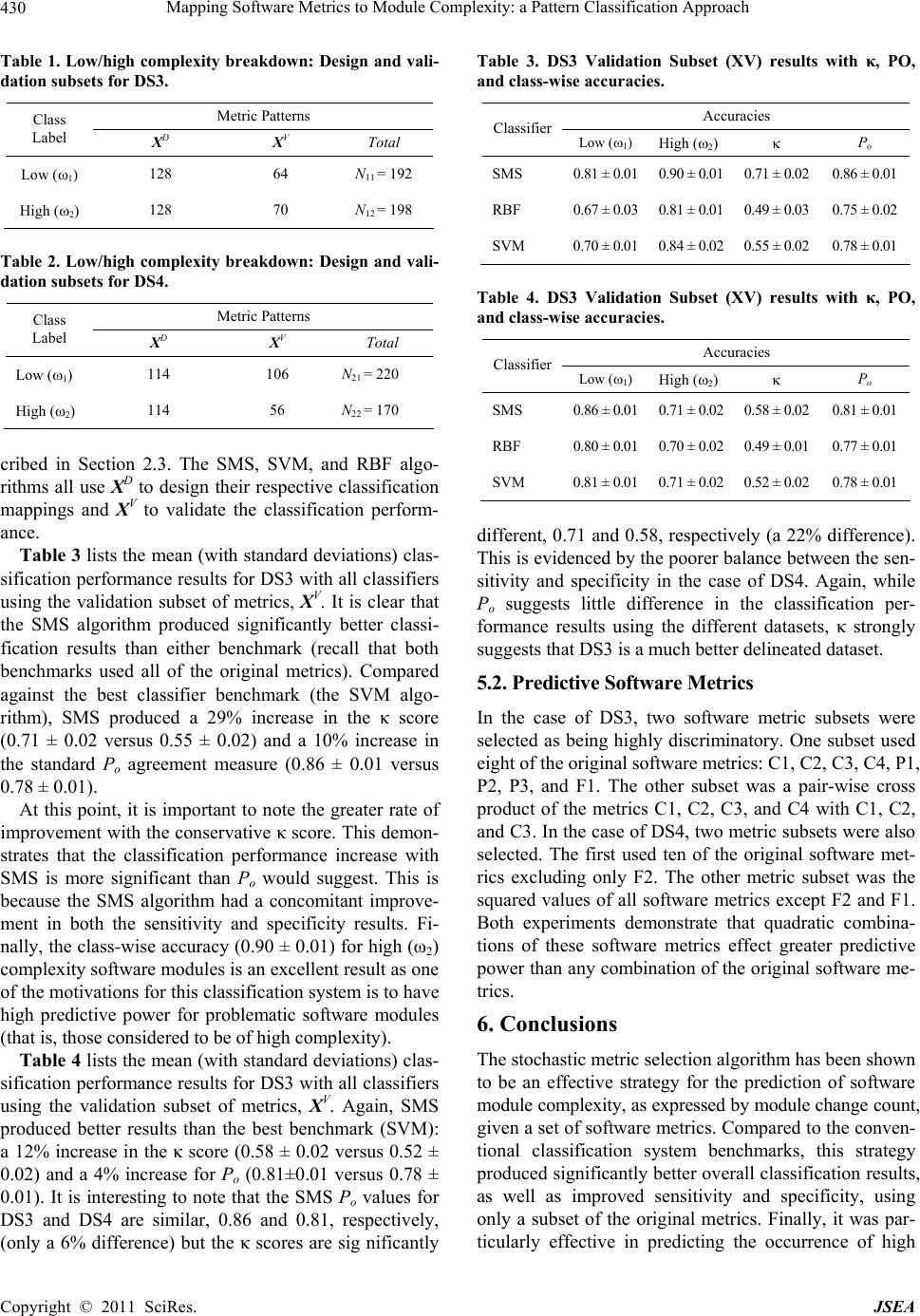

Mapping Software Metrics to Module Complexity: a Pattern Classification Approach 430
Table 1. Low/high complexity breakdown: Design and vali-
dation subsets for DS3.
Metric Patterns
Class
Label XD XV Total
Low (1) 128 64 N11 = 192
High (2) 128 70 N12 = 198
Table 2. Low/high complexity breakdown: Design and vali-
dation subsets for DS4.
Metric Patterns
Class
Label XD XV Total
Low (1) 114 106 N21 = 220
High (2) 114 56 N22 = 170
cribed in Section 2.3. The SMS, SVM, and RBF algo-
rithms all use XD to design their respective classification
mappings and XV to validate the classification perform-
ance.
Table 3 lists the mean (with standard deviations) clas-
sification performance results for DS3 with all classifiers
using the validation subset of metrics, XV. It is clear that
the SMS algorithm produced significantly better classi-
fication results than either benchmark (recall that both
benchmarks used all of the original metrics). Compared
against the best classifier benchmark (the SVM algo-
rithm), SMS produced a 29% increase in the κ score
(0.71 ± 0.02 versus 0.55 ± 0.02) and a 10% increase in
the standard Po agreement measure (0.86 ± 0.01 versus
0.78 ± 0.01).
At this point, it is important to note the greater rate of
improvement with the conservative κ score. This demon-
strates that the classification performance increase with
SMS is more significant than Po would suggest. This is
because the SMS algorithm had a concomitant improve-
ment in both the sensitivity and specificity results. Fi-
nally, the class-wise accuracy (0.90 ± 0.01) for high (ω2)
complexity software modules is an excellent result as one
of the motivations for this classification system is to have
high predictive power for problematic software modules
(that is, those considered to be of high complexity).
Table 4 lists the mean (with standard deviations) clas-
sification performance results for DS3 with all classifiers
using the validation subset of metrics, XV. Again, SMS
produced better results than the best benchmark (SVM):
a 12% increase in the κ score (0.58 ± 0.02 versus 0.52 ±
0.02) and a 4% increase for Po (0.81±0.01 versus 0.78 ±
0.01). It is interesting to note that the SMS Po values for
DS3 and DS4 are similar, 0.86 and 0.81, respectively,
(only a 6% difference) but the κ scores are sig nificantly
Table 3. DS3 Validation Subset (XV) results with κ, PO,
and class-wise accuracies.
Accuracies
Classifier
Low (1) High (2)  Po
SMS 0.81 ± 0.010.90 ± 0.01 0.71 ± 0.02 0.86 ± 0.01
RBF 0.67 ± 0.030.81 ± 0.01 0.49 ± 0.03 0.75 ± 0.02
SVM 0.70 ± 0.010.84 ± 0.02 0.55 ± 0.02 0.78 ± 0.01
Table 4. DS3 Validation Subset (XV) results with κ, PO,
and class-wise accuracies.
Accuracies
Classifier
Low (1) High (2)  Po
SMS 0.86 ± 0.010.71 ± 0.02 0.58 ± 0.02 0.81 ± 0.01
RBF 0.80 ± 0.010.70 ± 0.02 0.49 ± 0.01 0.77 ± 0.01
SVM 0.81 ± 0.010.71 ± 0.02 0.52 ± 0.02 0.78 ± 0.01
different, 0.71 and 0.58, respectively (a 22% difference).
This is evidenced by the poorer balance between the sen-
sitivity and specificity in the case of DS4. Again, while
Po suggests little difference in the classification per-
formance results using the different datasets, κ strongly
suggests that DS3 is a much better delineated dataset.
5.2. Predictive Software Metrics
In the case of DS3, two software metric subsets were
selected as being highly discriminatory. One subset used
eight of the original software metrics: C1, C2, C3, C4, P1,
P2, P3, and F1. The other subset was a pair-wise cross
product of the metrics C1, C2, C3, and C4 with C1, C2,
and C3. In the case of DS4, two metric subsets were also
selected. The first used ten of the original software met-
rics excluding only F2. The other metric subset was the
squared values of all software metrics except F2 and F1.
Both experiments demonstrate that quadratic combina-
tions of these software metrics effect greater predictive
power than any combination of the original software me-
trics.
6. Conclusions
The stochastic metric selection algorithm has been shown
to be an effective strategy for the prediction of software
module complexity, as expressed by module change count,
given a set of software metrics. Compared to the conven-
tional classification system benchmarks, this strategy
produced significantly better overall classification results,
as well as improved sensitivity and specificity, using
only a subset of the original metrics. Finally, it was par-
ticularly effective in predicting the occurrence of high

Mapping Software Metrics to Module Complexity: a Pattern Classification Approach431
complexity modules, which is an important characteristic
for software project managers and program developers
when maintaining and updating software modules.
7. Acknowledgements
The author would like to thank A. Demko and C. Wiebe
for their valuable contributions in implementing the sto-
chastic metric selection algorithm in Scopira. The author
would also like to thank M. R. Lyu for making the MIS
dataset available for this pattern classification investiga-
tion.
This work was supported in part by the Natural Sci-
ences and Engineering Research Council of Canada
(NSERC).
REFERENCES
[1] S. R. Chidamber and C. F. Kemerer, “A Metrics Suite for
Object-Oriented Design,” IEEE Transactions on Software
Engineering, Vol. 20, No. 6, 1994, pp. 476-493.
doi:10.1109/32.295895
[2] B. A. Kitchenham, R. T. Hughes and S. G. Kinkman,
“Modeling Software Measurement Data,” IEEE Transac-
tions on Software Engineering, Vol. 27, No. 9, 2001, pp.
788-804. doi:10.1109/32.950316
[3] N. E. Fenton and A. A. Kaposi, “Metrics and Software
Structure,” Information and Software Technology, Vol.
29, No. 6, 1987, pp. 301-320.
doi:10.1016/0950-5849(87)90029-2
[4] N. E. Fenton and M. Neil, “A Critique of Software Defect
Prediction Models,” IEEE Transactions on Software En-
gineering, Vol. 25, No. 5, 1999, pp. 675-689.
doi:10.1109/32.815326
[5] G. Poels and G. Dedene, “Distance-Based Software
Measurement: Necessary and Sufficient Properties for
Software Measures,” Information and Software Technol-
ogy, Vol. 42, No. 1, 2000, pp. 35-46.
[6] E. J. Weyuker, “Evaluating Software Complexity Meas-
ures,” IEEE Transactions on Software Engineering, Vol.
14, No. 9, 1988, pp. 1357-1365. doi:10.1109/32.6178
[7] M. Reformat, W. Pedrycz and N. J. Pizzi, “Software
Quality Analysis with the Use of Computational Intelli-
gence,” Information and Software Technology, Vol. 45,
No. 7, 2003, pp. 405-417.
doi:10.1016/S0950-5849(03)00012-0
[8] G. A. F. Seber, “Multivariate Observations,” John Wiley
& Sons Ltd., Hoboken, 1984.
doi:10.1002/9780470316641
[9] R. O. Duda, P. E. Hart and D. G. Stork, “Pattern Classifi-
cation,” 2nd Edition, Wiley-Interscience, New York, 2000.
[10] R. Gnanadesikan, “Methods for Statistical Data Analysis
of Multivariate Observations,” 2nd Edition, John Wiley &
Sons Ltd., New York, 1997. doi:10.1002/9781118032671
[11] N. J. Pizzi and W. Pedrycz, “Effective Classification Us-
ing Feature Selection and Fuzzy Integration,” Fuzzy Sets
and Systems, Vol. 159, No. 21, 2008, pp. 2859-2872.
doi:10.1016/j.fss.2008.03.015
[12] M. R. Lyu, “Data Directory in the CD-ROM,”
http://www.cse.cuhk.edu.hk/~lyu/book/reliability/data.ht
ml
[13] J. C. Munson and T. M. Khoshgofthaar, “Software Met-
rics for Software Reliability Assessment,” In: M. R. Lyu,
Ed., Handbook of Software Reliability Engineering,
McGraw-Hill, New York, 1996, pp. 493-529.
[14] R. Lind and K. Vairavan, “An Experimental Investigation
of Software Metrics and Their Relationship to Software
Development Effort,” IEEE Transactions on Software
Engineering, Vol. 15, No. 5, 1989, pp. 649-653.
doi:10.1109/32.24715
[15] R. S. Pressman and R. Pressman, “Software Engineering:
A Practitioner’s Approach,” McGraw-Hill, New York,
2000.
[16] N. E. Fenton and S. L. Pfleeger, “Software Metrics: A
Rigorous and Practical Approach,” PWS Publishing,
Boston, 1997.
[17] J. F. Peters and W. Pedrycz, “Software Engineering: An
Engineering Approach,” John Wiley & Sons Ltd., Hobo-
ken, 1999.
[18] M. H. Halstead, “Elements of Software Science,” Elsevier,
New York, 1977.
[19] T. J. McCabe, “A Complexity Metric,” IEEE Transac-
tions on Software Engineering, Vol. 2, No. 4, 1976, pp.
308-320. doi:10.1109/TSE.1976.233837
[20] E. K. Tang, P. N. Suganthan and X. Yao, “Gene Selection
Algorithms for Microarray Data Based on Least Square
Support Vector Machine,” BMC Bioinformatics, Vol. 7,
No. 95, 2006. doi:10.1186/1471-2105-7-95
[21] Q. Liu, A. Sung, Z. Chen and J. Xu, “Feature Mining and
Pattern Classification for LSB Matching Steganography
in Grayscale Images,” Pattern Recognition, Vol. 41, No.
1, 2008, pp. 56-66.
[22] N. Kasabov and Q. Song, “DENFIS: Dynamic Evolving
Neural-Fuzzy Inference System and Its Application for
Time-Series Prediction,” IEEE Transactions on Fuzzy
Systems, Vol. 10, No. 2, 2002, pp. 144-154.
doi:10.1109/91.995117
[23] B. Schölkopf and A. J. Smola, “Learning with Kernels:
Support Vector Machines, Regularization, Optimization,
and Beyond,” MIT Press, Cambridge, 2002.
[24] V. Vapnik, “Statistical Learning Theory,” John Wiley &
Sons Ltd., New York, 1998.
[25] L. Wang, “Support Vector Machines: Theory and Appli-
cations,” Springer-Verlag, Berlin, 2005.
[26] V. Vapnik and A. Lerner, “Pattern Recognition Using
Generalized Portrait Method,” Automation and Remote
Control, Vol. 24, 1963, pp. 774-780.
[27] W. H. Press, S. A. Teukolsky, W. T. Vetterling and B. P.
Flannery, “Numerical Recipes: The Art of Scientific
Computing,” 3rd Edition, Cambridge University Press,
Cambridge, 2007.
[28] J. Moody and C. J. Darken, “Fast Learning Networks of

Mapping Software Metrics to Module Complexity: a Pattern Classification Approach 432
Locally–Tuned Processing Units,” Neural Computation,
Vol. 1, No. 2, 1989, pp. 281-294.
[29] S. M. Weiss and C. A. Kulikowski, “Computer Systems
that Learn: Classification and Prediction Methods from
Statistics, Neural Nets, Machine Learning and Expert
Systems,” Morgan Kaufmann Publishing, San Mateo,
1991.
[30] B. S. Everitt, “Moments of the Statistics Kappa and
Weighted Kappa,” British Journal of Mathematical and
Statistical Psychology, Vol. 21, 1968, pp. 97-103.
[31] J. L. Fleiss, “Measuring Agreement between Two Judges
on the Presence or Absence of a Trait,” Biometrics, Vol.
31, No. 3, 1975, pp. 651-659. doi:10.2307/2529549
[32] T. McGinn, P. C. Wyer, T. B. Newman, S. Keitz, R.
Leipzig and G. Guyatt, “Tips for Learners of Evi-
dence-Based Medicine: 3. Measures of Observer Vari-
ability (Kappa Statistic),” Canadian Medical Association
Journal, Vol. 171, No. 11, 2004, pp. 1369-1373.
doi:10.1503/cmaj.1031981