Applied Mathematics, 2011, 2, 854-865
doi:10.4236/am.2011.27115 Published Online July 2011 (http://www.SciRP.org/journal/am)
Some Applications of Optimal Control in Sustainable
Fishing in the Baltic Sea
Dmitriy Stukalin, Werner H. Schmidt
Institut für Mathematik und Informatik, Greifswald, Germany
Received April 18, 2011; revised May 19, 2011; accepted May 22, 2011
Abstract
Issues related to the implementation of dynamic programming for optimal control of a three-dimensional
dynamic model (the fish populations management problem) are presented. They belong to a class of models
called Lotka-Volterra models. The existence of bionomic equilibria will be considered. The problem of op-
timal harvest policy is then solved for the control of various classes of its behaviour. Therefore the focus will
be the optimality conditions by using the Bellman principle. Moreover, we consider a different form for the
optimal value of the control vector, namely the feedback or closed-loop form of the control. Academic ex-
amples are studied in order to demonstrate the proposed methods.
Keywords: Optimal Control Problems, Maximum Principle, Piecewise Constant Optimal Control, Bellman
Principle
1. The Problem
Currently the fish populations in the Baltic Sea have
many problems, which are mainly caused by hu man in-
fluence. Some fish species are catched too much. The
fundamental risk of overfishing is that a stock (occur-
rence of species in a given region) is so decimated that
the natural regeneration ability is not given and at worst
the species die out. The Living Planet Index for marine
species of the WW F shows an average decrease of 14%
between 1970 and 2005 (see Living Planet Report
2008). The over fishing is the main cause apart from
possible environmental factors (climate change, pollut-
ants, etc.).
Therefore, the goal of the Baltic Sea fishermen must
be conscientious, by the policy prescribed regulations
and the advance (such as from International Council for
the Exploration of the Sea) to protect the Baltic Sea
fauna deal. A responsible management must reduce the
fishing effort to an environmentally acceptable level and
call for the cooperation among the participating countries.
This is of utmost importance, since the economic value
of the catches depends on the stock and the biodiversity
of the Baltic Sea.
Several interacting species are modeled, which inhabit
in a common habitat with limited resources. So, a dy-
namic system is to be studied, which depends on several
states and controls (e.g. the number of fishing boats). A
typical question for such systems is to find a controller
that regulates the system in a desired target. In many
applications a cost functional is to be optimized, this is
usually a functional of the state trajectory and the con-
trols of the system. The profit of a sustainable fishing
industry should be maximized without disappearance of
the species.
In this paper necessary (and sometimes sufficient) op-
timality conditions are derived. Numerical methods are
obtained from the optimality conditions in order to cal-
culate (approximately) optimal controls.
2. Optimal Control P r o b l e m s
Whenever a state function depending on the time is de-
scribed by an ordinary differential equation which de-
pends on the con trol variable, it is called a control system
of ordinary differential equations. Optimal control is
related to the development of space flight and military
researches beginning from the 1950s. We can find the
applications of the control theory in economics, in
chemistry or even in population dynamics. The general
task of optimal control is defined as follows:
Let m R

 be a nonempty (often convex and
closed) control region. Let ,,
g
qf be given smooth

D. STUKALIN ET AL. 855
functions:
1
:
:
:.
n
nn
n
qR R
f
RR R
g
RR R



A continuous and piecewise continuously differenti-
able function (state function) as well as a
piecewise continuous (or piecewise constant) function
(control function) are called admissible, if
the ODE
(): RRn x
(): Ru
 

 

0
00
,,,
x
tftxtut ttT
xt x



is valid. We are looking for admissible pairs


x

,


u

which maximize an objective (cost) functional of Bolza
type:
      
0()
,, d,ma
T
u
t
Jugtxt uttqTxTx

 
 (1)
Often the optimal control can be calculated by me-
thods using the Pontryagin maximum principle or by
solving the Hamilton-Jacobi-Bellman equation.
3. Extended Lotka-Volterra Models with M
Populations
A logistic model of development for a two-population
system can be written in the following form [1,2]. Let be
12
,

 growth coefficients, 12 ,


the phagos coeffi-
cients and 12 ,
K
K given numbers (capacities or logisti-
cal terms). We denote the population sizes as 1
x
and
2
x
.
The differential equatio ns for th e development of the
populations are
  
  
1
111 12
1
2
222 21
2
1
1
xt
x
txtxt
K
xt
x
txt xt
K












 
 













We denote generally:
i

are growth coefficients, ij

are the phagos coef-
ficients of the population i with respect to the population
j and Ki are logistical terms.
We denote the control of the fish populations


i
ut
(it can be a regulation of the fishing, e.g. the number of
the fishing boats if ), pi are fish prices (per
ton), ri are catch proportionalities. Therefore, the devel-
opment of m populations can be described by a general-
ized system

i
ut N
 




 
1
1mj
ii
iii ij
j
ii
i
ii
i
j
x
t
xt xt
xt xt
K
KK
xt
utrdK









where


0
0
ii
x
x

are given for
1,, .im
The objective function (the profit) is to be maximized
 
()
11
0
() max
Tmm
t
i
ii iiu
ii
i
xt
Jupu trdcdu te
K
 








under the restrictions


max
0,1,,;0
i
utuimt T.

 
c are the cutter costs per day and d is the number of
days in which we catch. If we calculate the present value
of future profits, we consider a discount rate t
e


. This
plays an important role in economic models.
4. Bellman’s Principle
A key aspect of dynamic programming is the Bellman
principle. The basic idea is to calculate the optimal solu-
tions of many small subproblems and then to compose
these subsolutions to a suitable global optimal solution. It
was formulated in 1957 by Bellman.
An optimal policy has the property that whatever the
initial state and initial decision are, the remaining deci-
sions must be an optimal policy with regard to the state
resulting from the first decision [3].
This idea can be used to derive a necessary and suffi-
cient condition. We consider here two forms of the opti-
mal controls of (1), namely the open-loop form and the
closed-loop form. The closed-loop form gives
the optimal value of the control vector as a function of
the time and the current state. The form of the optimal
control vector derived via the necessary conditions is
called open-loop. However, even though the closed-loop

ˆ,utx


ˆ,u

 and open-loop


*
u controls differ in form,
they yield identical values for the optimal control at each
date of the planning horizon. It follows




t
*
ˆ,utx



*
ut.
The open-loop form gives the optimal value of the
control vector as a function of the time and the initial
values of the state vector. The closed-loop form of the
optimal control is a decision rule, for it gives the optimal
value of the control for any current period and an admis-
sible state in the current period that may arise. In contrast,
the open-loop form of the optimal control is a curve, for
it gives the optimal values of the control as the inde-
pendent variable time over the planning horizon.
We consider an optimal control problem (1) under the
control condition:





0
,,,
m
utRtt Tu

  is piecewise con-

D. STUKALIN ET AL. 856
tinuous. st function The co



0
,:, n Vtx tTRR is defined
as
,
(2)
where
:
    
()
,max ,,d,
T
ut
Vtxg xuqTxT  



 

:, m utTR is admissible in


,tT and

x
 is the corresponding trajectory with

x
tx

.
ective

,tx gives the optimal value of the o fuVbjnc-
tion starting from the time


0,ttT and the starting
point x, followi ng the ODE.
We define the Hamiltonian H as









,,, ,,,H txuVtxgtxuV,,,
xx
txftxu
Necessary condition e value function to the
prAssume there exists th

,Vtx
oblem (1) in


0,n
tT R and this function is continu-
ously differentia
Let *()u be an o
ble. pen-loop optimal solution of (1).
Then thrresponding closed-loop solution ˆ(,)u
e co

 sat-
isfies the condition

ˆ, argmautx 
 
x,,,, ,n
x
uH txuVtxxR  
and


0,ttT
and

,Vtx is a solution of the PDE:
   

   
0
,, ,
,,.
tx
u
V txtt T
V TxTqTxT

 

max ,,, ,H txuVtx
Proof:

is the cost function for the part of

,txt t
the solution, that beg

Vt ins at the time tt with state

x
tt .
Then for 0tT t it is:




Since V is assumed to be continuous differentiable and
g

,tx
 



()
max , ,d,.
tt
u admissiblet
V
gx uVttxtt
 



  



to be continuous,
  
,, d
tt
x u
t
g


 can be ap-

proximated for every continuity point t of ()u

as
 


,,
g
txt uttot ,where ∆t is sufficientlyll. sma
It follows:
 



 


()
,max,,
,(
u admissible
xgtxt utt
Vt txttt


  ,
where represents the higher order terms, that
Vt
()ot
means

0
lim 0
t
ot.
t
 
ing to Taylor’s theorem it is: Accord










 
,,,
,
t
x
Vt txttVtxtVtxt t
V txtxttot

 

  
Substituting this result into the previous equation and
using


,,
x
ftxu
, it follows for the partial
di0t
fferential equation



  

   

0max ,
,,,.
x
, ,t
u
0
g
txt uV
 txt
Vtxtftxtu t


 (3)
We can write the PDE (3) as

 
,max,,,,VtxHtxuVtx

,
x
(4)
because
t
u


,Vtx
n does not depend on u. The conditio boundary







,,xT qTxTV T follows
(4) is the Hamilton-Jacob
volution equation with a fin
immedi-
ately.
The PDEi-Bellman equation.
It is an eal condition. The
global solvability, assumed in the first definition, is not
assured in general1.
Sufficient condition
If it’s given on


0,n
tT R

a real, continuously dif-
ferentiable function


,tx, wh
equation
Vich satisfies the Hamil-
ton-Jacobi-Bellman



 
, ,,,,
tx
u
V txtxuVtx


 
max
,,
H
VTxTqTxT (5)
and if the control



ˆ,argmax ,,,,
x
u
utxH txuVtx



(6)
(depending on t and x) is admissible, then
sponding open-loop controlwith the cthe corre- orrespond- *()u
ing state trajectory *()
x

is an optimal solution of (1).
Proof:
Since the left-hand e is independent from u, (5) can
bermed into: sid transfo




max,, , ,,0.
tx
uVtxH txuVtx  



(7)
*()u

and We choose admissible open-loop controls
()u

on


0,tT.
Let *()
x

and ()
x


be the unique state trajectory,
h are atewhicnerand in ged by *()u ()u


0,tT, so
that




00
.
*0
x
tx
tx

 Then it m :
follows fro(6) and (7)
1The name refers to William Rowan Hamilton (1805-1865), who
contributed to the developmen t of the calculus of variations, to
Carl Gustav Jacobi (1804-1851), who studied the theory of sufficient
conditions in the calculus of variations, and to Richard Bellman
(1920-1984), who brough t the dynamic programming on the way.
By the way, this equation comes from Constantin Carathéo dory
(1873-1950), whose name was not men tioned.

D. STUKALIN ET AL. 857
x
With the definition of the Hamiltonian

 


 

*** *
0, ,,,,
,,,,.
t
txH txtutVtx
xtutV tx
 
 
,
tx
V
VtxH t



x
H
gV f 
and taking into account
 

d,,, ,,
d
VtxVtx Vtx
f
txu


tt x
that this inequality can be written as
  

 


*
** d,
0,,d
,.
d
Vtx
gtx t utt
x
t


We integrate this inequality over the interval
d
,, Vt gtxt ut




0,tT
and obtain

,
by using
  



0
0
** *
00
,,,d,
T
t
t
Vt xgtxtuttqTx T

 



,, d ,
Tgtxtutt qTxT
 


 

   
0
00
d,,,,,
d
T
t
VVTxTVt xVTxTqTxT
t 


.
was added on both sides. Since

00
,Vt x ()u

s them
is arbi-
alue of the objective functional i maxi-
he control [4,5].
5. Algo
o formulate a construc-
tive algorithm:
trary the v
mized by t*()u
rithm
Now we can use this therem and
1) Identify


 
,, ,,, ,,
f
txugtxuq xt
fic problem. with the
mizing value
functions of a speci
2) Write down the corresponding Bellman equation.
3) Calculate ˆ uas function of

ˆ
,, :,,.
xx
txV utxV
from

ˆ,,
4) Add the ma

xi
x
utxV in the
right-hand side of the Bellman equatio-
mby usin
We mpare this mod with knods
n. (PDE)
5) Solve the Bellman equation. (analytically or nu
erically)
6) Compute ** (), ()xu
for 0
ttT g 3.
6. An Example. The Comparison with
Methods Using the Maximum Principle
want to coethwn metho
based on the Pontryagin maximum principle.
Let us consider the problem:
 
,
x
txtut 


0
0,
x
x ()u
piecewise constant
 
12
11
1min 
2
0
d
22
Ju ttx 
 (8)
A necessary optimality condition for (8) is the maxi-
necessary conditions were developed
by Pontryagin and his co-workers in Moscow in the
1950s. They introduced the idea of adjoi
append the differential equation to the objective func-
tio
conditions that the adjoint function should
sa
mum principle. The
nt functions to
nal [6].
Note that, the adjoint functions hav e a similar purpose
as Lagrange multipliers in multivariate calculus, which
append constraints to the functions of several variables to
be maximized or minimized. Thus, one begins by finding
appropriate
tisfy.
Let ** (), ()xu

 be optimal, then there is a nontrivial
solution of the adjoint equation
 

**
,,,,tHtxtutt
x



 so that for almost
all t












** *
,,, max,,,,
u
H
tx t u ttHtx t ut 



and the transversality condition

q
tT
x


.
In our example it is

 is sat-
isfied
 
2
1
,,,
H
2
txuux u 


sequently and con

,Ht

,, 0.xu u
u





That means




*
ut t  
in the profo r almost all t. cess equation, we obtain a
y value problem:
Replacing this
two-point boundar



 
, 0,
0
x
txttxx   

 
, 1t t

,,,1.Htxu x
x
 




The solutions of these equations a re:
 
121
1
, , 01.
2
ttt
tCextCe Cet 


  
The initial condition 210
2
1
CC x and the final con-
dition

1
21
1
12 C eCeCe 

  
1
give the constants
C1, C2:
2
00
12
23
.
22
,
13 13
x
x
ee


Therefore, it follows the open-loop-solution
e
CC

D. STUKALIN ET AL. 858
 
2
**
00 0
2
2
.
13
t
2
3
,
13
tt
x
exe
xt ut
ee




ellman principle provides the same solution in
another way:
Find the function such that
xe
(9)
The B

,,Vtx
   
2
1
,1, 1 1VTxVxqxx 

 

2
,m
ax,,,,.
tx
u
VtxHtxuVtx


Due to
 
2
1
,,, 2
xx
H
txuVuVx u  the nec-
esr a ma H in sary condition foximum ofuR

is

,,, 0.
x
HtxuV
u


This is exactly satisfied when
x
uV, that means

ˆ,,
x
x
utxV V. We have in mind . Therefore, UR
 
2
1
ˆˆ
,,, .

2
xxxx
H
HtxuVVVx V
this t
has the form:
The Hamilton-Jacobi-Bellman equation for ask
2
1
2
txx
VxVV
 
.
We use the ansatz because the
objective function, as quation with
respect tu

2
,,VtxAt x
well as the process e
o are polynomial. Then it follows

2
x
22
,.
13 t
Vt
xe


Therefore,
 
22
ˆ,13
xt
utxVe 
By using the differential equation the open-
2
, .
x
tx
loop solu-
tion can be calculated. It is
 


0
22
2, 0.
13 t
xt
x
txtx x
e
 


and this initial value problem has the solution

2
*00
2
3.
13e
With respect to

tt
xe xe
xt





**
ˆ,ut utx we obtain the opti-
mal control

*02
2
13
t
x
e
ut e as a func-tion of the time t.
Control Problems w ith Piecewise Constant
Controls
Now we consider problem (1) with piecewise constant
controls.
th of the intervin
-
ble.
7. Closed-Loop Optimality Conditions for
If the lengal is fixed, the Pontryag
maximum principle in the classical form is not applica
There is an alternate Pontryagin-like-way. Let


*t u


kk
uut be optimal on


1
,
kk
tt
. Then it follows:
1k
t
H


  

*
,,,d
uk
t
txtuttt  0, (10)
e Bellman principle we can also win optimal-
ity
k
Using th
conditions. Let be 01n tt t  predetermined
time points and ()
x

absolutely continuous.
The problem is now:
 
1 1k
t
n
k
 
 
0,,
,max
k
kt
nn u
J
ugttdt
 
xtu
qt xt











 (11)
The process equation is:








,,,
k
xtf txtut
 if

1kkk
k

,), 0,1,,1.tT ttn

 The optimal control


*
k
t uu

is to be found.
At first we consider the special case n = 1 (one control
interval).
We denote


0
ut v

and define the new
tion
for the process, which starts at
value func-
 

,, ,Wtxvg x  





1
11
, d,
t
t
v qtxt   
time t with the vector


x
tx

d witand is performeh the constant control
v

. This function W is continuously differentiable in
t and x. It is not to be confused with the function V
(chapter 4), sins no maximum operator.
We can form necessary conditions [7].
Ne
ce here i
ulate new
cessary condition
Let


,,Wtxv be continuously differentiable i t and
x. Let n


ˆ,utx be
e process an optimal constant control that leads th



 



,,,,
x
tf txtutxxtx


 from x
on


1
,tt . The control ˆ u is constant also in


01
,tt.
control Then this


ˆ,utxsatisfies for all


01
,ttt the
condition




00 00
ˆˆ
,,argmax,,utxut xWt xv
v
here


,,Wtxv satisfiwes the partial differential equa-
tion:





,, ,,,,, WtxvWtx,, v
f
.
txv g
in other words,
txv
tx



v 

D. STUKALIN ET AL. 859
 




1
0

,,,, ,,,, ,
,,,
n
i
ii
n
xvWtxv ftxvgtxv
tx
txvt tR





1
and
Wt





111
,,,, .Wtxv qtxtv 
Proof:
The proof is similar to the previous one.

,is the cost function for the part
starts at the time with state


,Wttxt

t v
of the solution, that

tt
x
tt under the infl
It is obviously: uence of the co
Since W is assumed to be continuous diferentiable
an
ntrol v.
 



,,,,d,,,
.
tt
t
WtxvgxvWt txt tv
v
 

 



f
d g to be continuous,
 
,,d
t
gx v
tt


 can be ap-
proximated as



,,

g
txt vtot. ows:




, ,,xt vt Wttxt
It foll



,,Wtxvgt

represents the higher order terms, that mean

,
.
t v
ot



ot s

00
ot
t

.
According to Taylor’s t
lim
t
heorem we obtain:
   

 
   
,, ,, ,,
,,.
x
W ttxttvWtxtvWtxtvt
Wtxtvxt tot
  


t

Substituting this result into the previous equation,t
follows with i

,,
x
ftxv
 the PDE
,
   
0,, (,,
t




,, ,,
x
g
txt vWtxt v
Wt xtv ftxtv
or in another form
 

,,,, ,,,,. WtxvWtxv
f
txv gtxv
tx



In the special problem it is 
so

The boundary condition
 
0,,,,JvWtxvv
the optim al contr ol vect o r c an be obt ained by

max,Wt x

00 00
ˆ,arg,
v
ut xv







11
,, ,Wtxv qtxt
1
follows immediately.
trol intervals the definition of neces-
alogous. Let be
In case of n con
sary conditions is an




01 1
,,,
n
utv vv


v
The function
with .,0,,1
k
vk n 


,,Wtxv is for all


1,,1 kk
ttt kn

 
defined as:
 

,,,, d
k
t
t
Wtxvg xv

 
d for all


1, nn
ttt

 as:

n
t

an




,,,, d,.
nn
t
Wtxvgxvqt xt   

It follows for all


1,,1 k
t
k
tt kn


:









 

1111
ˆˆ , argmax
,
v
utxutx W
Wtx



,,, ,
,,, ,,,,,
kk kk
ttxt v
vWtxv ftxv gtxv
tx
 

 





 
,Wt qt x

ˆ
0, ,, ,,,1,
0, ,,.
kkk
nn
WtxvWt xut xkn
xv v


 

8. Open-Loop Optimality Conditions for
Control Problems w ith Piecewise Constant
We can also formulate the optimality conditions for te
problem (11) in open-loop form. Let
Controls
h

,
x
tv be a solu-
tion of the process equatio n






1
,,,,,, ,
kk
xtv ftxtvvtvtt
t
,

 

with




,
kk
x
tv xt for , for all 0, ,1kn 
v

 and 00 ()
x
tx

.
The Hamiltonian is:



,,,,,
H
txv gtxv  


,,
f
txv . We consider the special case n = 1 (one
trol interval)
 
con.
Necessary condition in open-loop form
Let ** (), ()xu

 be optimal with



*
0,t ut
*
u






**
0
,
x
txtut, then it is



 


*000
argmax ,,,
v
utStvtvxt 


0

where


,tv  is a soluf tion o
 
 

,,
,,,
tvH txt
x
tvt t

  
01
,,,,,v vtv 


 

(12)
and


,Stv is a solution of





 


,,
,,,,, ,
Stv H tv
t
Htxtv vtv
,,,,txtv v
x
tv
x






(13)


D. STUKALIN ET AL. 860
with

00

0
,
x
tv
xt x and the transversality condi- tions
 


11
1
,
,qtxt tv
x



and
 

 

11
11
,
,,
qt xt
Stvxtvqtxt
11
,
x

 

are satisfied for all
Proof:
nsider the equatio
.v
We con (13):
 

 


,,,,,,
,,,,,,
Stv Htxtv vtv
t
Htxtv vtv
x
tv
x






is equivalent to

 
  

,,,,,,
,,,,,,.
Stv gtxvtvf txv
t
Htxtv vtv
x
tv



 

It follows fro m (12)
x


   
,,, ,, ,,. Stv
g
txvtvxtvtvxv
t


 



We integrate this equation over
t


1
,tt :
   

1
11
,, ,,d,
,,.
t
t
StvStvgxvtv xtv
tv xtv
 




1
t
1
,
From the previous we obtain



,,d
t
gxv



the transversality
  
11
,, ,Wtxvqtxt
co and from nditions
 

 

 
11
,,tv xtv xt   


11
1111
11
,
,,,
,.
qt xt
Stvxtvqt xt
x
qt

 

It follows:
,
n ir

because is constant. It follows with
. 
the right-hand side of the equation is the
function of We obtain the open-loop form:
  
 
,,,,, ,
,,,.
StvWtxvtv xtvWtxv
Stvtv xtv




As shown the pevious chapter it is

ˆ
u
 
00 00
ˆ
,,arg max,,
v
txutxWtx v



ˆ,utx

  
00
0000 0
,:
ˆ,argmax,,
v
xt vxt
utxSt vt vxt 



The term on
0.t



 


*000
argmax ,,
v
utStvtvxt 


0
.
nition of neces-
sary conditions is analogous.
We have to maximize:
n
In case of n control intervals the defi
 




1
0,,d,
k
t
n
kn
kt
1k
J
ugtxtuttqtx







 t
under the constraint:




 



00
 
1,
,,,
,.
kk k
k
x
tftxtutttt
xtx ut




**
(), ()xu

 be optimal with



**
,
k
ut ut Let






**
,k
x
txtut, for 0, ,1,kn

then it is






*argmax ,
k
ut St,
k
u tuxt  ,
k
u k

where


,Stv is a solution of

 

  

,,,,,,
,,,,, ,
Stv Htxtv vtv
t
Htxtv vtv
x
tv
x






(14)
and



,tv  is a solution of
 
,,H tv
x




1
,,,,,
,, ,
kk
tvtxtv v
tvt t




 

(15) 
with




 

 

 

000
*1
*
*
,,
,0,
0,, ,
0,, ,
kkkk
kkk
kkk
xt vxtx
xt vxtxtut
tv tut
StvSt ut






,
he tran ns and tsversality conditio





 

 

,
,,
,
,,
nn
n
nn
nn
qt xt
tv x
qt xt
St vxtqtxt
x




 

nn
are satisfied.
9. An Example. The Multistage Open-Loop
Control
We want to solve a two stages-optimal control problem.

D. STUKALIN ET AL. 861
Let be


0,1t and 01 0,tt0.5.
 
01
0.5 ,0.5;1TT
We obtain two
time The process
equation is:
intervals:
 
0; .







0
,0,1;0
k,
x
txtutkx x 
 6)
piecewise constant:
(1
()u
  



 

 

 
1
1
01 01
122
22
0
,,,
0,,
11
d1min
1
d1
22
k
k
t
k
kt
ututv v
ututT
Jvtx
vtx






 


v
v
)
The Hamiltonian is
0
1
0.5 ,,utut T (17
0
1
22
1max
k
k
k
kt
t
J

 
v
v
v
ut 

2
1.,,, 2
H
txv x  
The r the problem (17) are:
(18)
, (19)
and it is
v v
necessary conditions fo

 
**
1
0.5
argmax0.5,0.5,0.5,,
v
uu
Sv vxv




 
**
00
0argmax0,0,
v
uuSvvx 


 
 
11
2
11
1,1, ,
1
1,1, ,
2
vxv
Sv xv

 

v
v 
It follows for 0,1i:
 
 
2
,,,
ii
tv tv  

1
,,
2
ii ii
St vtv vv  

and
 
  
00 10
,,,
0,,0.5,0.50,
iii
xtvxtvv
x
vxx vxv
 

 (20)
The transition conditions are:
The solutions of the ODE




*
01
*
01
0.50,0.5,,
0.50.5,.
vu
vSu
 
 0,S



,,
iii
x
tvxtv v 

0,1i are
0
1
,
.


01 0
12 1
,,
,,
t
t
x
tvA evtT
x
tvA evtT


 
 
According to

0
0
x
x we obtain 00vx
1
A


and with (20)



0 00.5 1
.
20
A
xvvve Therefore,
 


 
 
0.5
10001 1
10.5
100011
0.5
100 0
1, ,
0.5,
t1
,,,
x
tvxvvvee vtT
xvxve vve
xvxvev




 
 
v
and


1
,,
t
i
tv Ce   0,1.i

final cT 1 delivers he ondition fo r t =






11
10
00 01 1
1, 1,vCex
.5
x
vev vev



 
v
anonstant re, d gives us the c.
1
C Therefo
 


1
1
,,
t
i
tvve e 

 
21.5
00 01
0,1.
x vevve
i



1
tT

It follows for :



2
1111
12
1 1
1
,,
21.
2
t
Stvtv vv
21 .5
0001 1
x
vev veve

  ve v
  


The solution of this equation is:
 


21.5
100011
1
1
,
2
t
Stvx vev veveve

 
We obtain from the final condition:

2
12
1.vt C
2
C
 


 
1
10
1, vx0.52
0011112
2
210.5
00 01 1
1
2
11
10, .
22
SvevvevvvC
xxvevvev








v
Due to (18):



 




 





0 .52
000
()





**
1.512 0.52
000
2
210.5
000
1
1.51 0.5
00 0
0.5
00 0
0.5, 0.5,
1
argmax 4
11 ()
22
()
v
u vxv
1
0.5argmax 0.5,
v
u Sv
x
vvev vvevev
vxvevvev
xvevve ve
xvev

 







  

 
 
This is exactly satisfied when (with differentiation
ov itution
xv vevvvev

 

 
er v and subst*
00
vu

:



0.5* 0.5
00
*10.5 1.5
1
21212
42 3.

x
eue
ue ee
e


 (21)
Analogically, we obtain for 0:tT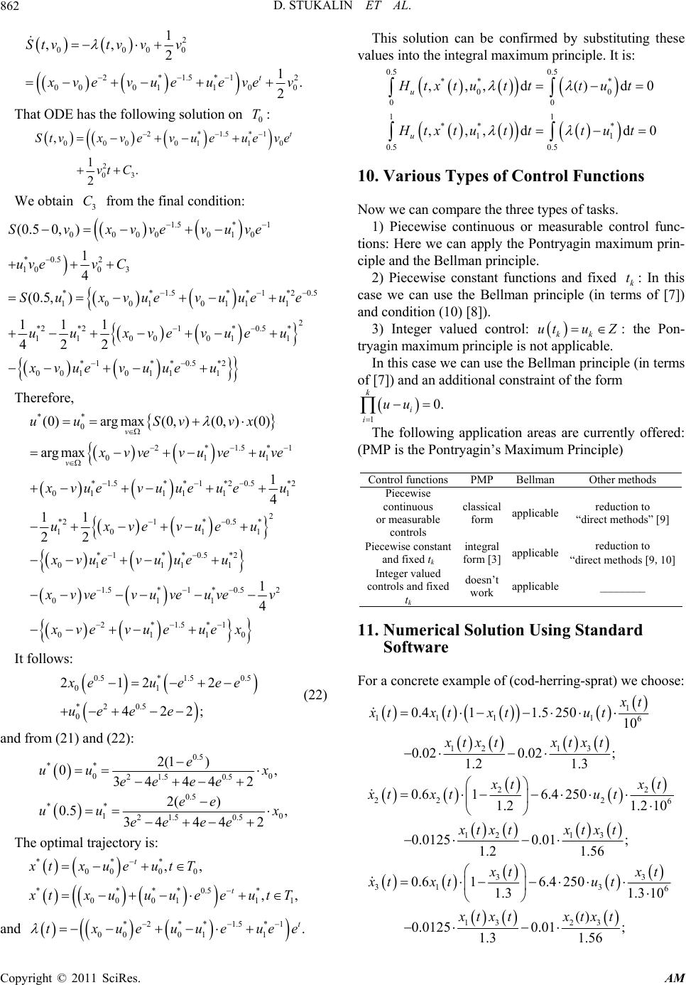

D. STUKALIN ET AL. 862




2
0000
2*1.5*1
00011 00
1
,,
21.
2
t
Stvtv vv
2
x
vev ueue vev


 
 

0:T That ODE has the following solution on
 


2*1.5*1
000 0110
2
03
,
1
.
2
t
Stvxv evu eueve
vt C

 

We obtain from the final condition:
3
C









*2 *2
11 00
422
uu xveu

 






10 0 3
**1.5*
1001 01
2
1* 0.5*
011
*1* *0.5*2
0010111
4
(0.5,)
111
S
Suxv uevu u
v eu
xvuevuueu


 

 
Therefore,
1.5* 1
0000 010
*0.5 2
(0.50,)
1
vxv vevuve
uvev C




* 1*20.5
11
eu e










*2 1* 0.5
10 1
11






**
2*1.5*1
011
* 1.5** 1*20.5*2
011111
2
*
1
*1* *0.5*2
0111 1
1.5 *
01
(0)argmax(0, )(0, )(0)
argmax
1
4
22
v
uuSvvx
0v
x
vvev uveuve
x
vuevuueu eu
xvuevuueu
xvvevuve

 




 


 
 
ux vevueu

  


 

1*0.5 2
1
2*1.5*1
0110
1
4
uve v
xve vueuex



 
It follows:


0.5*1.50.5
01
*2 0.5
212 2
422;
0
x
eueee
e ee
 
  u (22)
and from (21) and (22):


0.5
**
0
21.50.5
0.5
**
1
0
2 1.50.5
2(1 )
0
34 442
2( )
0.5 ,
34 442
e
uux
ee ee
ee
uu x
ee ee

 


 

The optimal trajectory is:
0
,





***
000 0
****0.5*
00011 1
,,
,,
t
t
xtxueutT
x
txuuueeutT



 
and e

This solution can be confirmed by substituting these
values into the integral maximum principle. It is:
0
0


10. Various Types of Control Functions
Now we can compare the three types of tasks.
1) Piecewise continuous or measurable control func-
tions: Here we can apply the Pontryagin maximum prin-
ciple and the Bellman principle.
e constant functions and fixed : In this
case we can use the Bellman principle (in terms of [7])
and condition (10) [8]).
3) Integer valued control: : the Pon-
the Bellman principle (in terms
of [7]) and an additional constraint of the form

 

*2**1.5 *1
00011.
t
txueuueue 

  
 

 



0.5 0.5
** *
00
00
11
** *
11
0.5 0.5
,,,d()d
,,,dd
u
u
Htxtuttt ut
Htxtuttt ut






2) Piecewis k t

kk
utu Z
tryagin maximum principle is not applicable.
In this case we can use

1
0.
k
i
i
uu




The following application areas are currently offered:
(PMP is tmum Principle)
Control funct ionsPMP Bellman Other methods
he Pontryagin’s Maxi
Piecewise
continuous
or measurable
controls
classical
form applicable reduction to “direct methods” [9]
Piecewise constant
and fixed t
integral
form [3]applicable reduction to “direct methods [9,10]
k
Integer valued
controls and fixed
tk
doesn’t
work applicable ________
11. Numerical Solution Using Standard
Software
For a concrete example of (cod-herring-sprat) we choose:
 




 
    
 
  
1
111 1
6
0.411.525010
xt
xtxtxtut
12 13
xt
x txtxt
22
22
0.02 0.02 ;
1.2 1.3
0.6 16.4 2
3
250 1
1.56
6
12 13
1.2.210
0.01250.01 ;
1.2
3
31 3
0.6 16.4 2506
1.3 1.3 10
x
txt
xt xtut
xtx txtxt
x
txt
xt xtut

 






 







 



13 23
()
0.01250.01 ;
xtxt xtxt

1.3 1.56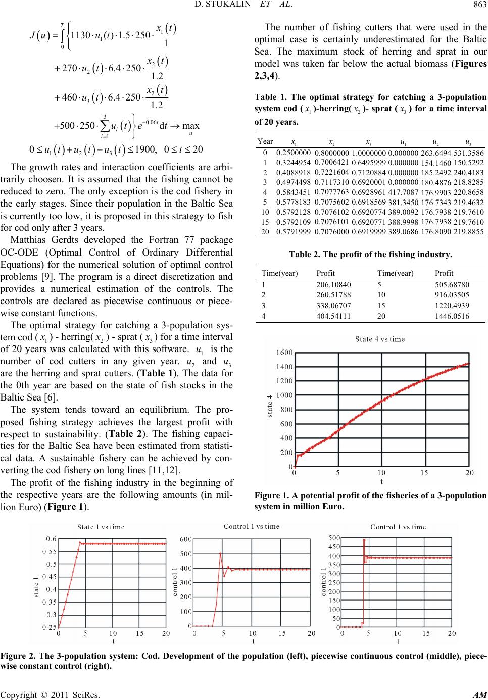

D. STUKALIN ET AL. 863
 
 
 


1
1
2
30.06
1
3
1130( ) 1.52501
1.2
6.4 2501.2
d
1900
t
i
xt
Ju ut
xt
ut
ut et
ut

 
 

 

 
es incoeffi arbi-
trarily choosen. It is assumed that the fishing cannot be
ery in
the Since their population in the Baltic Sea
is currently too low, it is proposed in this strategy to fish
Matthias Gerdts developed the Fortran 77 package
OC-ODE (Optimal Control of Ordinary Differential
Equations) for the numerical solution of optimal control
problems [9]. The program is a direct discretization and
provides a numerical estimation of the controls. The
controls are declared as piecewise continuous or piece-
wise constant functions.
The optimal strategy for catching a 3-population sys-
tem cod (

1
0ut

250
i
ut



0
2
2
2706.4250xt
ut


 
3
2
and
460
500max
u
, 020 t 
T




The growth ratteraction cients are
reduced to zero. The only exception is the cod fish
early stages.
for cod only after 3 years.
1
x
) - herri ng(2
x
) - sprat (3
x
) for a time interval
of s calculated wiware. is the
number od cu any n year. and
are the herring and sprat cutters. ().e data fo
the 0th year are based on the state of fish stocks in the
Baltic Sea [6].
The system tends toward an equilibrium. The pro-
posed fishing strategy achieves the largest profit with
respect to sustainability. (Table 2). The fishing capaci-
ties for the Baltic Sea have been estimated from statisti-
cal data. A sustainable fishery can be achieved by con-
verting the cod fishery on long lines [11,12].
The profit of the fishing industry in the beginning of
the respective years are the following amounts (in mil-
lion Euro) (Figure 1).
w the actual biomass (Figures
2,
20 years wa
of cth this soft give
Table 1
1
u
2
tters inu
Th3
u
r
The number of fishing cutters that were used in the
optimal case is certainly underestimated for the Baltic
Sea. The maximum stock of herring and sprat in our
model was taken far belo
3,4).
Table 1. The optimal strategy for catching a 3-population
system cod (1
x
)-herring( 2
x
)- sprat (3
x
) for a ti intervl
of 20 years.
Year 1
me a
x
2
x
3
x
1 u 2 u 3 u
00.2500000 0.
1
2
3
4
5
10
15
0.3244954
0.4088918
0.4974498
0.5843451
0.5778183
0.5792128
0.5792109
8000000
0.7006421
0.7221604
0.7117310
0.7077763
0.7075602
0.7076102
0.7076101
1.0000000
0.6495999
0.7120884
0.6920001
0.6928961
0.6918569
0.6920774
0.6920771
0.000000
0.000000
0.000000
0.000000
417.7087
381.3450
389.0092
388.9998
263.6494
154.1460
185.2492
180.4876
176.9903
176.7343
176.7938
176.7
531.3586
150.5292
240.4183
218.8285
220.8658
219.4632
219.7610
2938 219.7610 00.5791999 0.70760000.6919999 389.0686 176.8090 219.8855
Table 2. The profit of the fishing industry.
Time(year) Profit Time(year) Profit
1
2
3
4
206.10840
260.51788
338.06707
404.54111
5
10
15
20
505.68780
916.03505
1220.4939
1446.0516
Figure 1. A potential profit of the fisheries of a 3-population
system in million Euro.
Figure 2. The 3-population system: Cod. Development of the
wise constant control (right). population (left), piecewise continuous control (middle), piece-

D. STUKALIN ET AL. 864
Frt of the population (left), piecewise continuous control (middle),
pi
igue 3. The 3-populationen-system: Herring. Developmen
ecewise constant control (right).
Figure 4. The 3-populationen-system: Sprat. Development of the population (left), piecewise continuous control (middle),
piecewise constant control (right).
12. Comments
The value function is globally continuously
differentiable only inonal cases (for example, in
n operate even if the value
function is only piecewise differentiable. This happens
when the set of the points of discontinuity of is
composed of smooth surfaces.
Useful general principles that guarantee a -solution
of the HJB equation are not known. In generl, the value
function is not smooth. Even if the value function is
smooth, then the solution can be not expressed in explicit
formulas [13].
There is a possibility of introducing a generalized so-
lution concept, which is also obtained in the case of
non-differentiability of a value function.

,Vtx
excepti
the linear-quadratic problems).
The Bellman principle ca
V
1
C
a
This solution concept should be so general that it can
also be applied when the derivative


Dv x does not
exist for all n
x
R. On the oth
2003.
er haould be
ken so that onee does not get too many possible solu-
tions of the HJB quation - in the ideal case, the optimal
value function is the unique solution [14,15]. This gener-
alized solution is called a viscosity solution.
11. References
[1] M. Begon and M. Mortimer, “Populationsökolog
New York, 1956.
[3] M. Papageorgiou,“Optimierung,” R. Oldenbourg Verlag,
München, 1996.
[4] L. Grüne, “Modeling with Differential Equations,” Lec-
ture Notes, University of Bayreuth, 2003.
[5] T. Christiaans, “Neoklassische Wachstumstheorie,” Books
on Demand, Norderstedt, 2004.
[6] M. Brokate, “Control Theory,” Institute of Informatics
and Mathematics, Technical University of Munich, Mu-
nich, 1994.
[7] A. Pantelejew and A. Bortakovskij, “Control Theory
Examples and Practices,” Vysshaya Shkola, Moscow,
[8] W. H. Schmidt, “Durch Integralgleichungen Beschrie-
bene Optimale Prozesse mit Nebenbedingungen in Bana-
chräumen-Notwendige Optimalit ätsbedingungen,” Journal
of Applied Mathematics and Mechanics, Vol. 62, No. 2,
1982, pp. 65-75. doi: 10.1002/zamm.19820620202
nd, it sh
ta
ie,” Spe-
ktrum Akademischer Verlag, Heidelberg, 1997.
[2] A. J. Lotka,“Elements of Mathematical Biology,” Dover,
in
[9] M. Gerdts, “Optimal Control of Ordinary-Differential

D. STUKALIN ET AL. 865
Equations,” University of Hamburg, Hamburg, 2006.
[10] W. Alt, “Nichtlineare Optimierung: Eine Einführung in
Theorie, Verfahren und Anwendungen,” Viewer and
teubner Verlag, Wiesbaden, 2002.
[11] R. Döring, “Die Zukunft der Fischerei im Biosphären-
reservat Südost- Rügen,” Peter Lang GmbH, Frankfurt,
2001.
[12] P. Ernst and W. Müller, “Die Deutsche und Internationale
Dorschfischerei in der Ostsee im jahr 1998,” Informa-
tionen für die Fischwirtschaft aus der Fischereiforschung,
Vol. 46, No. 3, 1999, pp. 32-35.
[13] M. Bardi, I. Capuzzo-Dolcetta, “Optimal Control and
Viscosity Solutions of Hamilton-Jacobi-Bellman Equa-
tions,” Birkhäuser, Boston, 1997.
doi:10.1007/978-0-8176-4755-1
[14] L. Grüne, “Viskositätslösungen von Hamilton-Jacobi-
Bellman Gleichungen: Eine Einführung,” Numerical Dyna-
mics of Control Systems, 2004.
[15] P. Lions, “On the Hamilton-Jacobi-Bellman Equations,”
Acta Applicandae Mathematicae, Vol. 1, No. 1, 1983, pp.
17-41. doi:10.1007/BF02433840
[16] O. Rechlin, “Fischbestände der Ostsee, ihre Entwicklung
in den Jahren seit 1970 und Schlussfolgerungen,” ihre
Nutzung, Rostock, 1999.