J. Biomedical Science and Engineering, 2008, 1 85-90
Published Online August 2008 in SciRes. http://www.srpublishing.org/journal/jbise JBiSE
Retrospective analysis of chronic hepatitis C in un-
treated patients with nonlinear mixed effects mod-
el
Jian Huang1, Kathleen O’Sullivan1, John Levis2, Elizabeth Kenny-Walsh3, Orla Crosbie3 & Liam Jo-
seph Fanning2
1 Statistical Consultancy Unit, University College Cork, Ireland. 2 Molecular Virology, Department of Medicine, Hospital Cork University, Ireland. 3 Depart-
ment of Gastroenterology and Hepatology, University Hospital Cork,Ireland. Correspondence should be addressed to Jian Huang ([e-mail]).
ABSTRACT
It is well known that viral load of the hepatitis C
virus (HCV) is related to the efficacy of interferon
therapy. The complex biological parameters that
impact on viral load are essentially unknown.
The current knowledge of the hepatitis C virus
does not provide a mathematical model for viral
load dynamics w ithin untreated patients. We car-
ried out an empirical modelling to investigate
whether different fluctuation patterns exist and
how these patterns (if exist) are related to host-
specific factors. Data was prospectively col-
lected from 147 untreated patients chronically
infected with hepatitis C, each contributing be-
tween 2 to 10 years of measurements. We pro-
pose to use a three parameter logistic model to
describe the overall pattern of viral load fluctua-
tion based on an exploratory analysis of the data.
To incorporate the correlation feature of longitu-
dinal data and patient to patient variation, we
introduced random effects components into the
model. On the basis of this nonlinear mixed ef-
fects modelling, we investigated effects of host-
specific factors on viral load fluctuation by in-
corporating covariates into the model. The pro-
posed model provided a good fit for describing
fluctuations of viral load measured with varying
frequency over different time intervals. The aver-
age viral load growth time was significantly dif-
ferent between infection sources. There was a
large patient to patient variation in viral load as-
ymptote.
Keywords: Logistic model, Viral load, Viral
genotype, Mixed effects modelling
1. INTRODUCTION
Approximately 3% of the world population is infected by
the hepatitis C virus (HCV). This virus is a single
stranded positive sense RNA virus and does not exist as a
single clonotype. It is found as a complex mixture of
similar but non-identical isolates, hence, quasispecies.
There are seven different genotypes of HCV each with a
unique population of subtypes. The nomenclature used to
describe these genotypes is numerical, while subtypes are
described alphabetically. The amount of virus present in
serum at any one time is referred to as the viral load,
which can be measured in serum by RT-PCR (a method
based on amplification of genomic RNA [1]). A wide
range of viral load fluctuation over time was observed
within some untreated patients [2]. Treatment efficacy is
reduced when viraemia is greater than 5.7-6.0 log10
IU/mL [3]. Knowledge of viral load fluctuations could
lead to a more optimised treatment initiation time point.
To date several studies have attempted to elucidate viral
load fluctuation within untreated patients. Halfon et al. [2]
showed that viral load fluctuation within untreated pa-
tients was significant. Arase et al. [4] illustrated the ratio
of the maximum viral load to the minimum viral load was
related to acute exacerbation. Pontisso et al. [5] demon-
strated that the mean difference between the maximum
viral load and minimum viral load was significantly dif-
ferent between normal transaminases and fluctuating
transaminases. Our previous studies [6, 7] have showed
that viral load does change over time in some patients and
exhibits periods of apparent stability in others.
The complex biological parameters that impact on
HCV viral load are essentially unknown. However, what
is known is that the magnitude of the viral load at any one
time represents the output of the equilibrium between
viral production and host mediated viral clearance. The
phenomenon of replicative homeostasis may explain viral
load fluctuation over time within an untreated patient [8].
Replicative homeostasis consists of a series of autoregula-
tory feedback epicycles that link RNA polymerase func-
tion, RNA replication and viral production and presents a
model which may rationalize why viraemia modulates
over time. Replicative homeostasis results dynamic equi-
librium controlled by the specificity of the interactions
between mutant or wild type envelope proteins and the
replicas, the RNA dependant RNA polymerase (RDRP).
In other words, a highly progressive RDRP exhibits a low
SciRes Copyright © 2008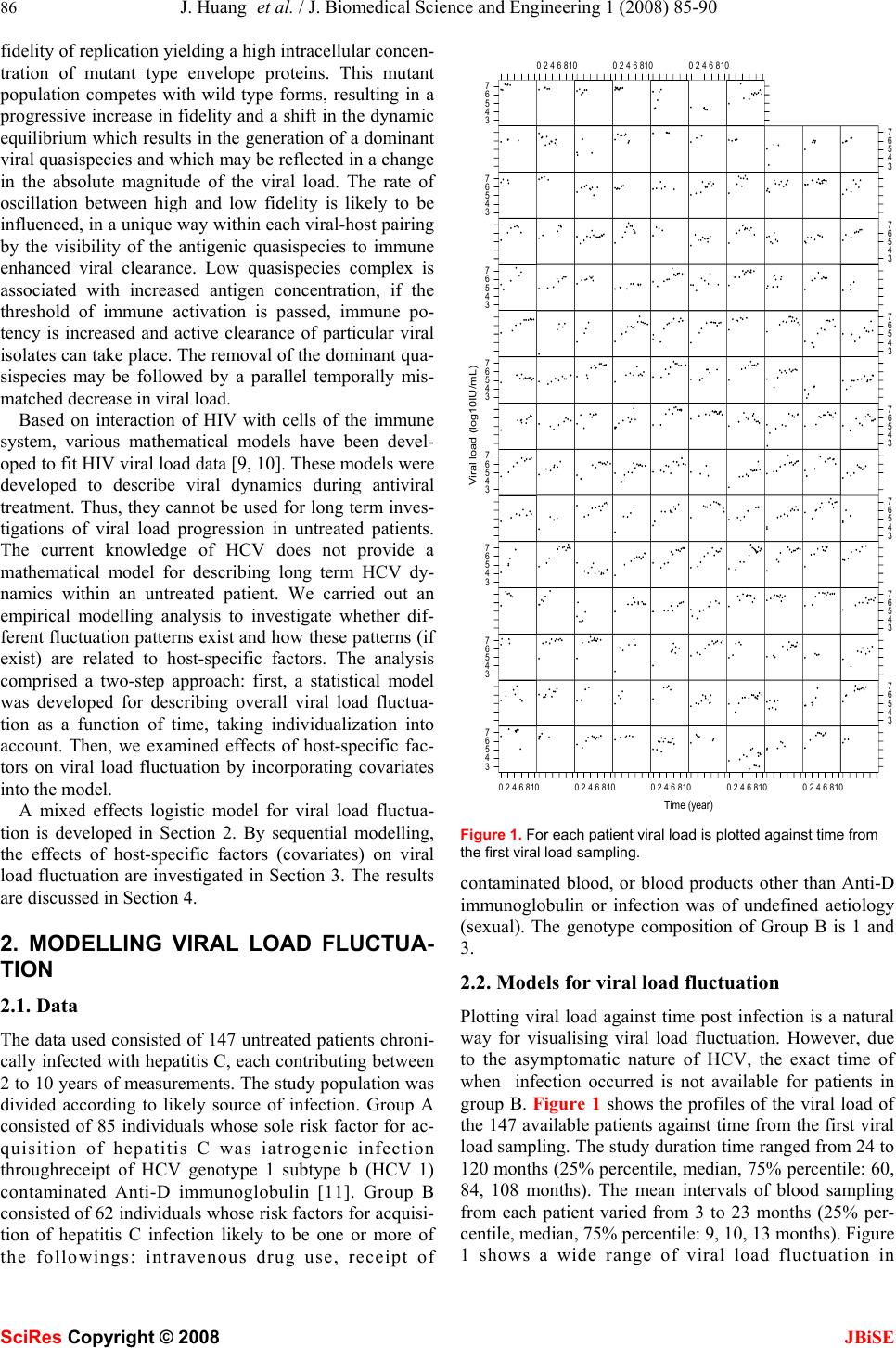

86 J. Huang et al. / J. Biomedical Science and Engineering 1 (2008) 85-90
SciRes Copyright © 2008 JBiSE
fidelity of replication yielding a high intracellular concen-
tration of mutant type envelope proteins. This mutant
population competes with wild type forms, resulting in a
progressive increase in fidelity and a shift in the dynamic
equilibrium which results in the generation of a dominant
viral quasispecies and which may be reflected in a change
in the absolute magnitude of the viral load. The rate of
oscillation between high and low fidelity is likely to be
influenced, in a unique way within each viral-host pairing
by the visibility of the antigenic quasispecies to immune
enhanced viral clearance. Low quasispecies complex is
associated with increased antigen concentration, if the
threshold of immune activation is passed, immune po-
tency is increased and active clearance of particular viral
isolates can take place. The removal of the dominant qua-
sispecies may be followed by a parallel temporally mis-
matched decrease in viral load.
Based on interaction of HIV with cells of the immune
system, various mathematical models have been devel-
oped to fit HIV viral load data [9, 10]. These models were
developed to describe viral dynamics during antiviral
treatment. Thus, they cannot be used for long term inves-
tigations of viral load progression in untreated patients.
The current knowledge of HCV does not provide a
mathematical model for describing long term HCV dy-
namics within an untreated patient. We carried out an
empirical modelling analysis to investigate whether dif-
ferent fluctuation patterns exist and how these patterns (if
exist) are related to host-specific factors. The analysis
comprised a two-step approach: first, a statistical model
was developed for describing overall viral load fluctua-
tion as a function of time, taking individualization into
account. Then, we examined effects of host-specific fac-
tors on viral load fluctuation by incorporating covariates
into the model.
A mixed effects logistic model for viral load fluctua-
tion is developed in Section 2. By sequential modelling,
the effects of host-specific factors (covariates) on viral
load fluctuation are investigated in Section 3. The results
are discussed in Section 4.
2. MODELLING VIRAL LOAD FLUCTUA-
TION
2.1. Data
The data used consisted of 147 untreated patients chroni-
cally infected with hepatitis C, each contributing between
2 to 10 years of measurements. The study population was
divided according to likely source of infection. Group A
consisted of 85 individuals whose sole risk factor for ac-
quisition of hepatitis C was iatrogenic infection
throughreceipt of HCV genotype 1 subtype b (HCV 1)
contaminated Anti-D immunoglobulin [11]. Group B
consisted of 62 individuals whose risk factors for acquisi-
tion of hepatitis C infection likely to be one or more of
the followings: intravenous drug use, receipt of
Time (year)
Viral load (log10IU/mL)
3
4
5
6
7
02468100246810024681002468100246810
3
4
5
6
7
3
4
5
6
73
4
5
6
7
3
4
5
6
73
4
5
6
7
3
4
5
6
73
4
5
6
7
3
4
5
6
73
4
5
6
7
3
4
5
6
73
4
5
6
7
3
4
5
6
73
4
5
6
7
3
4
5
6
7
024681002468100246810
Figure 1. For each patient viral load is plotted against time from
the first viral load sampling.
contaminated blood, or blood products other than Anti-D
immunoglobulin or infection was of undefined aetiology
(sexual). The genotype composition of Group B is 1 and
3.
2.2. Models for viral load fluctuation
Plotting viral load against time post infection is a natural
way for visualising viral load fluctuation. However, due
to the asymptomatic nature of HCV, the exact time of
when infection occurred is not available for patients in
group B. Figure 1 shows the profiles of the viral load of
the 147 available patients against time from the first viral
load sampling. The study duration time ranged from 24 to
120 months (25% percentile, median, 75% percentile: 60,
84, 108 months). The mean intervals of blood sampling
from each patient varied from 3 to 23 months (25% per-
centile, median, 75% percentile: 9, 10, 13 months). Figure
1 shows a wide range of viral load fluctuation in

J. Huang et al. / J. Biomedical Science and Engineering 1 (2008) 85-90 87
SciRes Copyright © 2008 JBiSE
0246810
34567
Tim e
log10.IU.per.mL
Lowess
logistic
quadratic
Figure 2. Scatter plot of viral load overlaid with the LOWESS,
logistic and quadratic fitted curves.
some untreated patients. In addition, the viral load pro-
files vary between patients. To identify an appropriate
model to describe the overall fluctuation of viral load as a
function of time, the locally-weighted polynomial regres-
sion smoothing (the R function LOWESS) was performed
on the data (Figure 2). The pattern obtained from the
LOWESS shows that viral load increase over some time
period, followed by a period of the more stabilized viral
load. Such patterns can be described by logistic models
[12]
,))/)81ln()(exp(1/( ijijij ty
ε
γ
β
α
+
−
−+= (1)
where ij y is the logarithm (base 10) of the measurement
of viral load for the ith patient at the jth measurement time
(from the first viral load sampling) ij t and the model er-
ror ij ε is assumed to be i.i.d. N (0,2 σ ). The parameter
α
is the asymptote (the limit of viral load growth),
β
is
the midpoint, the time when the most rapid viral load
growth occurs. The scale parameter
γ
is the growth time,
time interval during which growth progresses from 10%
to 90% of the asymptote [12]. )81ln( is introduced into
model (1) to facilitate interpretation of
γ
.
As a comparison we fed the quadratic polynomial
model to data as well. The fitted curves corresponding to
the quadratic polynomial model (AIC=2896.37) and lo-
gistic model (AIC=2896.01) are also shown in Figure 2.
As can be seen from Figure 2 both models captured the
basic structure of the LOWESS smooth with the logistic
one performing better at the tail. Having a smaller AIC
value the logistic model was selected to describe the
overall pattern of viral load fluctuation.
It is also evident from Figure 1 that there exists a large
patient to patient variation in viral load fluctuation. To
account for this patient to patient variation random com-
ponents were introduced into model (1) yielding the fol-
lowing mixed effects model
,)))/(ln(81)
))(((/(1)(
iji
iijiij r
btexpay
εγ
βα
++×
+−−++= (2)
where ),,( iii rba are assumed to be the i.i.d random vec-
tor, independent of the model errors and follow the nor-
mal distribution N(0,Σ).
α
is replaced by i a
+
α
to ac-
count for patient to patient variation in the viral load as-
ymptote.
α
is called the fixed effect and represents the
mean level of the viral load asymptote for the population.
i
a is called the random effect and represents the individ-
ual patient departure from the mean level. Similarly, the
fixed effects
β
and
γ
represent the mean levels of the
midpoint and growth time for the population, respectively.
The random effects i band i rare the individual patient
departures from the mean levels of the midpoint and
growth time, respectively.
The R package nlme [13] was used to fit nonlinear
mixed effects models. In model (2), all three parameters
consisted of a fixed effect term and a random effect term.
Such models might be over parameterized. In these cases,
the variance-covariance matrix of random effects become
seriously ill-conditioned, making convergence difficult or
impossible. We adopted model building strategies sug-
gested in [13] to determine an adequate but parsimonious
model.
We began with fitting model (2) to data. Convergence
was achieved. However, convergence was sensitive to
changes in the initial values and the algorithm failed to
converge using values slightly different from the fitted
values. Checking the fitted model we found that the esti-
mated covariance matrix
Σ
)
has off diagonal terms of
zero. Hence, we refitted model (2) with a diagonal co-
variance matrix
Σ
. Then the possibility of eliminating one
or more random effects from the model was investigated.
First, we compared models generated by eliminating one
of the three random effects from model (2) and found that
the model with random components in
α
and
β
had the
largest likelihood value, termed as model A. Then we
considered models generated by removing two of the
three random effects from model (2) and found that the
model with a random effect in
α
had the largest likeli-
hood value, termed as model B. To establish the signifi-
cance of random effects, we followed the procedure de-
scribed by Verbeke and Molenberghs [14], who provide
an outline for testing the need for random effects by com-
paring the log-likelihood between the nested models with
and without random effects. The asymptotic null distribu-
tion of the test statistics is a mixture of Chi-squares. The
results are summarised in Table 1. As can be seen from
the table there are significant random effects in
α
(P<0.0001) and
β
(P<0.0001). Model B was preferred.
Hence we re-parameterized model (2) as follows
ij
iijiij bty
εγ
βαα
+×
+−−++=
))/)81ln(
))((exp(1/()( (3)
When fitting model (3) to data, we estimate the stan-
dard deviations of the random effects as 0.63 (log10IU/mL)
and 1.32 (year) for the asymptote and midpoint of growth
time, respectively.
The time variable used in the model is the time from
the first viral load sampling. It may not be related to the
time since onset of infection. A patient can enter the study
at any time since onset of infection. For example, some

88 J. Huang et al. / J. Biomedical Science and Engineering 1 (2008) 85-90
SciRes Copyright © 2008 JBiSE
Table 1. Comparisons of nested models to establish significance
of random effects.
Random effects LR test P-Value
a Model (1) vs Model B <0.001
b Model A vs Model A <0.001
c Model A vs Model (2) Nonsignificant
may present two months after the time of infection; others
may present one year later. Such time differences can be
accounted for in the model by random effects in
β
. Ran-
dom effects in
β
allow the logistic growth curve to fit
viral load profiles measured at different time spans from
onset of infection. Significant patient to patient variation
in
β
(P<0.001) may reflect that patients may have en-
tered the study at different time from the times of infec-
tion. The significant random effects in
α
(P<0.001) indi-
cates that there exist large patient to patient variation in
the asymptote. However, from a clinical perspective our
current understanding of hepatitis C disease is such that
this variation is difficult to interpret with certainty.
3. ANALYSIS OF COVARIATES
In this section, we examined the effects of covariates on
the viral load fluctuation by sequentially incorporating
them into model (3). A similar approach has been used in
[15]. The covariates considered are viral genotype, gender,
infection source (Group A and Group B) and age (< 45
years verses ≥ 45 years). In model (3) there are three
fixed effects terms,
α
β
and .
γ
Any given covariate may
have a significant effect on at least one of the terms. For
example, gender had significant a effect on
γ
(P<0.05)
but not on
α
and .
β
When a covariate was incorporated
into the model only were significant terms retained. Inter-
actions were considered only if a fixed term was signifi-
cantly affected by at least two covariates. Initially, one
covariate was incorporated into model (3). Incorporating
age into model (3) failed to produce any significant term.
Hence, three one-covariate models were produced. The
one-covariate model with the maximum likelihood was
selected as the optimum one-covariate model. Subse-
quently, one of the remaining covariates was incorporated
into this model and yielded no significant term. The selec-
tion process was stopped. The process is summarized in
Table 2. The final model selected to fit the viral load data
is model (4) with
γ
influenced by infection source and
can be expressed as follows
,)))/()81ln(
))((exp(1/()(
ijr
iijiij btay
εγγ
βα
=+×
+−−++= (4)
where r
γ
represents infection source effect on the growth
time
γ
. The significance of this term was assessed using
the F-tests (P<0.0001).
As an alternative approach we incorporated covariates
into model (3) using the backward elimination approach.
The selection process began with incorporating all the
Table 2. Sequentially incorporating covariates into model (3) to
determine important covariates. Significant term is indicated in the
bracket.
Models P-value Log-
likelihood
Time (model (3)) -946.40
Time + gender (
γ
) <0.001 -931.34
Time + infection source (
γ
) <0.001 -925.63
Time + genotype (
γ
) <0.001 -946.01
covariates into model (3). Then non significant terms
were removed from the model recursively. Using a
significance level of 0.05, this approach also selected
model (4) as the final model.
A likelihood ratio test was used to test the difference be-
tween the fixed effects represented by model (3) and(4).
The result favors model (4) with P<0.0001.
Plotting the standardized residuals against the fitted
values of model (4) and the Normal plot of the residuals
(not shown) did not illustrate any concerns about the
model assumptions. The individual fitted curves (Figure
3) indicate good fits to the data, keeping in mind that the
data were irregularly and sparsely sampled.
The fitting of model (4) to the data is summarised in
Table 3. The results show that the mean viral load as-
ymptote for the population was 6.44 (log10IU/mL). The
most rapid viral load growth occurred, on average, 3.29
years before patients entered the study. The mean growth
time for the population was 11.04 years. The patients in
Group A experienced, on average, significantly longer
growth time (delta = 3.80 year) compared to those in
Group B.
Since all patients in Group A are female and have vi-
ral genotype 1, to separate the gender and genotype ef-
fects from the infection source effect, the previous ap-
proach to evaluating the effects of covariates by sequen-
tially incorporating them into model (3) was applied to
Group B. No significant one-covariate model was pro-
duced. This finding is very different from the results de-
scribed earlier. Using the full data we found that all co-
variates except age had a significant effect on viral load
growth pattern (see Table 2). One possible explanation is
that the gender and genotype significance found in the
previous analysis may be due to the significance of infec-
tion source. Another possibility is that number of patient
in Group B was small and there may have not been suffi-
cient power to identify gender and genotype significance.
4. CONCLUSIONS AND DISCUSSIONS
We have developed a mixed effects logistic model for
describing the viral load fluctuation within untreated pa-
tients with chronically infected HCV. The model’s diag-
nostic analysis indicated that the proposed model pro-
vided a good fit to the data. Due to the asymptomatic na-
ture of HCV, it is impossible to determine the exact time
when a patient was infected. Hence the time variable used
in the model is the time since an individual patient pre-

J. Huang et al. / J. Biomedical Science and Engineering 1 (2008) 85-90 89
SciRes Copyright © 2008 JBiSE
sented.
Table 3. The results of fitting model (4) to the data.
Terms Value Std.errors p-Value
α
: Grand mean 6.44 0.068 <0.0001
β
: Grand mean -3.290.223 <0.0001
γ
: Grand mean 11.040.750 <0.0001
γ
:Group B- Group A -3.800.444 <0.0001
Time (year)
Viral load (log10IU/mL)
3
4
5
6
7
02468100246810 024681002468100246810
3
4
5
6
7
3
4
5
6
73
4
5
6
7
3
4
5
6
73
4
5
6
7
3
4
5
6
73
4
5
6
7
3
4
5
6
73
4
5
6
7
3
4
5
6
73
4
5
6
7
3
4
5
6
73
4
5
6
7
3
4
5
6
7
02468100246810 0246810
Figure 3. Viral load is ploted against time from the first viral load
sampling, overplayed with the individual fitted curve (solid line),
for each of 147 patients.
Random effects in
β
allow the model to fit viral load
profiles beginning at different time from the time of in-
fection. As shown in Figure 3, partially measured viral
load profile can be fitted by the corresponding section of
the logistic growth curve.
Recently, Gray et al. [15] conducted an empirical mod-
elling of HIV-RNA viral load in vertically infected chil-
dren. They chose a linear model to represent the overall
pattern of HIV-RNA viral load among conventional poly-
nomials, change point models, and fractional models.
They compared various algorithms to fit the linear model.
Based on exploratory analysis of data we chose a nonlin-
ear model to describe the overall pattern of HCV viral
load within untreated patients. We investigated effects of
host-specific factors based on nonlinear mixed effects
models.
The quantification of viraemia is a snap shot in time of
the amount of virus present. The diurnal variation in viral
load is unknown; however, the amount of virus present at
any one time is the outcome of the equilibrium between
viral production (replication of genomic RNA and pro-
duction of infectious virions) and destruction of infected
hepatocytes. Although, there is considerable patient to
patient variation in viral load asymptote, from a clinical
perspective our current understanding of hepatitis C dis-
ease is such that these variations are difficult to interpret
with certainty. What is of interest is the difference in viral
load growth time. The growth time determines the
“speed” at which the asymptote is reached. A clinically
important parameter is the pre-treatment viral load. Viral
load has been established by numerous studies as an in-
dependent variable which determines outcome while on
anti-viral treatment. Patients with a viral load value below
6 log10 IU/mL are known to respond with higher efficacy
to therapy [3,16]. The difference in the growth time be-
tween groups A and B would indicate that more time
could be afforded to the pre-treatment assessment period
for group A while viral load remained within the range of
optimum efficacy.
The distinguishing feature of data presented here is the
longitudinal nature of the viral load measurement. Group
A represents a globally unique homogeneous cohort with
respect to the investigation of the natural history of hepa-
titis C infection. The empirical model proposed here is the
first attempt to describe long term viral load fluctuation in
untreated patients.
REFERENCES
[1] Fanning at el. (1999) Viral load and clinic pathological features of
chronic hepatitis C (1b) in a homogeneous patient population.
Hepatology, 29, 904-7.
[2] Halfon et al. (1998) Assessment of spontaneous fluctuations of
viral load in untreated patients with chronic hepatitis C by two
standardized quantitation methods: branched DNA and amplicor
monitor. J Clin Microbiol, 36(7), 2073–2075.
[3] Shiffman et al. (2007) Peginterferon alfa-2a and ribavirin for 16 or
24 weeks in HCV genotype 2 or 3. N Engl J Med,357(2), 124-34.
[4] Arase, Y., Ikeda, K., and Chayama, K. (2000) Fluctuation patterns
of HCV-RNA serum level in patients with chronic hepatitis C. J
Gastroenterol, 35, 221-225.
[5] Pontisso, P., Bellati, G., and Brunetto, M. (1999) Hepatitis C virus
RNA profiles in chronically infected individuals: Do they relate to
disease activity? Hepatology, 29, 585–589.
[6] Fanning et al. (2000) Natural fluctuations of hepatitis C viral load
in a homogeneous patient population: a prospective study.
Hepatology, 31, 225-9.
[7] Fanning et al. (2001) LA class II genes determine the natural
variance of hepatitis C viral load. Hepatology, 33, 224-30.
[8] R. Sallie. (2005) Replicative homeostasis II: influence of
polymerase fidelity on RNA virus quasispecies biology:
implications for immune recognition, viral autoimmunity and other
"virus receptor", diseases. Virol J, 22, 2-70,.

90 J. Huang et al. / J. Biomedical Science and Engineering 1 (2008) 85-90
SciRes Copyright © 2008 JBiSE
[9] Wu, H. (2005) Statistical methods for HIV dynamic studies in
AIDS clinical trials. Statistical Methods in Medical Research, 14,
171-192.
[10] Donnelly, C.A. and Cox, D.R. (2001) Mathematical biology and
medical statistics: contributions to the understanding of AIDS
epidemiology. Stat Methods Mes Res, 10(2), 141-54.
[11] Kenny-Walsh E. (1999) Clinical outcomes after hepatitis C
infection from contaminated anti-D immune globulin. Irish
Hepatology Research Group. N Engl J Med, 16, 1228-33.
[12] Meyer, P.S., Yung, J.W., and Ausubel, J.H. (1999) A Primer on
Logistic Growth and Substitution: The Mathematics of the Loglet
Lab Software. Technological Forecasting and Social Change, 61,
247-271.
[13] Pinheiro, J.C., and Bates, D.M. (2000) Mixed-Effects Models in S
and S-PLUS, Springer.
[14] Verbeke, G., Molenberghs, G. (2000) Linear Mixed Models for
Longitudinal Data. Springer, New York.
[15] L. Gray, M. Cortina-Borja and ML Newell. (2004) Modelling
HIV-RNA viral load in vertically infected children. Statist. Med,
23, 769-781.
[16] Zeuzem et al. (2006) Efficacy of 24 weeks treatment with
peginterferon alfa-2b plus ribavirin in patients with chronic
hepatitis C infected with genotype 1 and low pretreatment viremia.
J Hepatol, 44, 97-103.