Journal of Water Resource and Protection, 2015, 7, 769-780
Published Online July 2015 in SciRes. http://www.scirp.org/journal/jwarp
http://dx.doi.org/10.4236/jwarp.2015.79063
How to cite this paper: Khan, T.A. (2015) Groundwater Quality Evaluation Using Multivariate Methods, in Parts of Ganga
Sot Sub-Basin, Ganga Basin, India. Journal of Water Resource and Protection, 7, 769-780.
http://dx.doi.org/10.4236/jwarp.2015.79063
Groundwater Quality Evaluation Using
Multivariate Methods, in Parts of Ganga Sot
Sub-Basin, Ganga Basin, India
Taqveem Ali Khan
Department of Geology, Aligarh Muslim University, Aligarh, Ind ia
Received 6 May 2015; accepted 11 July 2015; published 14 July 2015
Copyright © 2015 by author and Scientific Research Publishing Inc.
This work is licensed under the Creative Commons Attribution International License (CC BY).
http://creativecommons.org/licenses/by/4.0/
Abstract
A quantitative analytical data from the alluvial aquifers of Ganga-Sot Sub-Basin (GSSB) is subjected
to multivariate statistical analysis in order to ascertain the groundwater quality characterization
depending on the top soil/physiographic divisions. The matrix consists of ten variables of 34
groundwater samples collected from evenly spaced locations. The Hierarchical cluster analysis
resulted in six clusters. Each cluster group is individually subjected to Principal component analy-
sis (PCA). PCA of group A explains cumulative variance of 83%, and 95% of group of B, 82% of
group C, 91% of group of D. Dissimilarity among the clusters is due to anthropogenic influence on
the groundwater regime. The PCA is done for the groundwater quality data of the whole area and
on the data of sub-divided area. The PCA of the whole area resulted in five components with cu-
mulative variance of 69.19%. The area is sub divided on the basis of soil type/physiography and
data falling in each sub-division is subjected to PCA. The PCA of clay loam soil/Ganga Mahwa low
land resulted in five PCs explaining cumulative variance of 91%. The PCA of sandy soil/central
upland data extracted four PCs with 80% of cumulative variance. The PCA of loam type of soil/Sot
plain extracted three PCs explaining cumulative variance of 91.751%. The three physiographic
units of the alluvium setting reflect distinct groundwater quality as manifested by the PCA. From
this study it can be ascertained that PCA can be used for the characterization of groundwater qual-
ity information.
Keywords
Principal Component Analysis, Hierarchical Cluster Analysis, Dendrogram, Aquifers
1. Introduction
Groundwater has taken the dominant place in India’s domestic and agriculture sector owing to its easy accessi-

T. A. Khan
770
bility. The last three decades has witnessed an unprecedented growth in the use of groundwater in the agriculture
sector. Groundwater now accounts for over 60 percent of the irrigated area in the country. India has seen an un-
precedented withdrawal of groundwater from 1960 to 2010 much higher than china and United States. This
sharp rise is attributed to the time when green revolution was set in motion [1]. In India, 80% of the domestic
supply is from groundwater in rural areas, where 2.8 - 3.0 million hand pumps operated boreholes have been
constructed in the past 30 years [2]. Development of gr oundwater resources and subsequent withdrawal to meet
the ever increasing demand has put the shallow aquifers in a depleting state. Decline of the groundwater table
has been observed in many parts of the western Gangetic plain. The average rate of decline is about 0.15 m/yr in
the western Ganges plains and in some places as high as 0.35 - 0.4 m/yr from 1994-2005 [3]. Su ch inter ference
altering the natural water balance has influenced the redox chemistry of the aquifer and solid-water interfaces
resulting in mobilization of several chemical contaminants present in the aquifer matrices as their natural con-
stituents [4]. Composition of groundwater in a region depends on the natural (such as wet and dry depositions of
atmospheric salts, evapo-transpir ation, soil/rock-water interactions) and anthropogenic processes which can alter
these systems by contaminating them or modifying the hydrological cycle [5].
Water quality depends on a variety of physico-chemical parameters and meaningful prediction, ranking anal-
ysis or pattern re cognition of the qu a lity of water requires multiv ariate projections methods for simultaneous and
systematic interpretation [6]. To deal with the multidimensional data and enable an overall evaluation of the
spatial variations in water quality, the multivariate techniques including cluster analysis and principal compo-
nent analysis (PCA) are often powerful methods [7].
Hierarchical cluster analysis is a powerful tool for analyzing water chemistry data [8]-[10] and has been used
to formulate geochemical models [11]. It is an exploratory data analysis tool used to sort out different objects
into groups. In clustering the objects are grouped such that the similar objects fall into the same class [12]. The
degree of association between two objects is maximal if they belong to the same group and minimal otherwise.
Hierarchical clustering joins the most similar observations and then successfully the next most similar observa-
tion. The levels of similarity at which observations are merged are used to construct a dendrogram [13]. The
Euclidean distance is represented on the horizontal axis of the dendrogram. It gives the similarity between two
clusters. The weighted pair group method was used and the Euclidean distance was selected as the measure of
similarity [14].
PCA can be used to reduce the dimensionality of the original data by extracting a smaller number of linear
combinations of the original variables i.e., principal components (PCs) that explain most of the variance of the
original data with minimal info rmation loss [15]-[17].
The Principal component analysis is used for data reduction and for deciphering patterns within large sets of
data [18] [19]. It extracts the eigenvalues and eigenvectors from the covariance matrix of original variables. The
numbers of factors, called principal components (PC), were defined according to the criterion that only factors
that account for variance greater than 1 (eigenvalue-one criterion) should be included. The rational for this crite-
rion is that any component should account for more variance than any single variable in the standardized test
score space [20]. The multivariate analysis is used in making the relationship between variables of the water
quality data. This technique aims to transform the observed variables to a set of variables, which are uncorre-
lated and arranged in decreasing order of importance. The principal aim is to simplify the problem and to find
new variables (principal c omponent s ) , whi ch make the da t a e a s i e r to u ndersta nd [21].
Multivariate statistical analysis is widely used to understand the natural and anthropogenic influence on
groundwater quality [22]-[24]. In most of the cases these techniques are applied to the water quality of the whole
area in order to asses trend detection, pollution source identification, optimization of water quality parameters
and water quality monitoring station s [25]-[30]. However, Qian et al. [7] used cluster analysis to group the sam-
pling sites and then carried a PCA on these clustered groups to ascertain the water qu ality characterization. The
objectives of the present study are to:
1) Characterize the groundwater quality, using multivariate s tatistica l analys is, in p ar ts of Gang a Sot Sub-basin,
Central Ganga Plain.
2) To test the hypothesis that if there is any influence of top soil/physiographic division in an alluvial setting on
the groundwater of an area. This has been tested in the following steps:
a) The matrix consist of 10 variables of 34 groundwater samples collected from locations evenly spaced in the
GSSB so as to cover the entire area.
b) PCA was done on the analytical data o f the whole area. Constituents with loadings >0.5 were considered as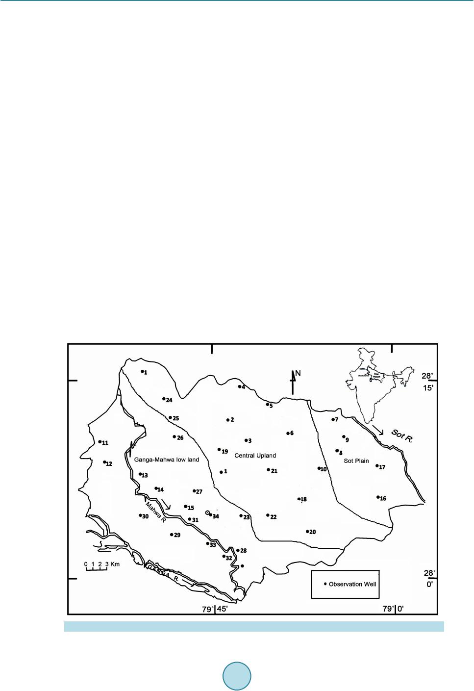

T. A. Khan
771
principal constituents .
c) Study area is sub-divided on t he bas is of top soi l/physiographi c division.
d) PCA is done separately on the analytical data falling in ea ch sub unit.
3) To explore the spatial variability in groundwater quality the difference in characteristics among different
sampling locations were determined by using clustering and the resultant clusters are individually sub jected
to PCA.
4) Relative importance of individual water quality variables were determined by PCA.
2. Site Description
The geomorphic setup of the Ganga Plain is believed to have evolved under changing conditions of climate, intra-
and extra-basinal tectonics and sea-level induced base-level changes [31]-[33]. River systems responded to all
these changes and evolved differentially in time and space [34]. The variations in the intensity of Indian mon-
soon apparently played a very significant role in the sedimentary processes that were additionally modulated by
tectonic-driven changes in the source and the sink regions. Early literature on the Ganga Basin identifies two
morphostratigraphic units, namely the Older Alluvium (Bhangar or Bangar) and the Newer Alluvium (Khadar)
[35]. The Older Alluvium comprises the higher interfluves areas while the sediments of major river channels and
their valleys constitu te the Newer Alluvium. The evolutio n of the aquifer in fluvial system is dependent upon the
hydrodynamics of the flow regime, geology and topography of the terrain leading to the terrigenous clastic de-
position system. These depositional systems are typically represented as the channel, flood plain and back
swamp deposits. The shallow character and high permeability of alluvial aquifers make them highly vulnerable
to contamination [36].
The Ganga Sot Sub-basin (GSSB) occupies about 1073 sq km in the central Ganga plain of vast Ganga basin
(Figure 1). It lies between the latitudes 27˚58' and 28˚17'N and the longitude 78˚35' and 79˚4'E. The River
Ganga and Sot form the southern and eastern boundaries, respectively, of the area while River Mahawa traverses
diagonally in the western part. The dominant land use in the area is composed of agriculture (82%), with barren
(2%), forest (2%) waste land (1%) fallow land (7%) and pastures (1%). The climate of the area is characterized
by cold winter with temperature falling to 5˚C and very hot summers with temperat ure rising 4 5˚C.
Figure 1. Base map of the study area showing sampling locations.

T. A. Khan
772
The aquifer of Ganga basin is considered to be one of the largest aquifer repositories of the world. The sedi-
ments in the Ganga basin were mainly derived from the fluvial agencies coming from the newly risen Himalayas.
Topographically, the area is a vast level expanse but its surface and appearance vary to a considerable extent and
is determined mainly by the course and character of the natural drainage channels. The slope of the country is
from north-west to south-east and this direction governs the course of the streams within the sub-basin.
Physiographically, the area can be divided into the three distinct physiographic units (1) Ganga Mahwa low-
land (2) Central upland (3) Sot plain.
2.1. Ganga Mahawa Lowland
Between the high ridge and Ganga river is the low-lying land which gently slopes due southeast. It is a broad
shallow depression representing a number of back swamps and abandoned channels. The area lying between the
Mahawa’s right bank and the Ganga, gently slopes towards the river Ganga. The soil is loam to clayey loam
which supports good crops.
2.2. Central Upland
It is a belt of high-land which runs through the centre of the study area, in a northwest to south east direction
forming a watershed between the Mahawa and the Sot rivers. The stretch is about 8 kms in width and consists
entirely of silt through fine to medium sands, which supports poor crops. There were number of springs along
the steep sided western margin of the upland. However, the eastern margin of the upland gradually slopes due
east and merges with the sot plain.
2.3. Sot Plain
This lies in the east of the upland—a broad, very gently sloping and perfectly homogeneous expense of good
fertile loam, varied only at places, by clay in the depression. The plain merges due east with the right bank of the
Sot river whi ch forms the eastern most boundary of the area.
3. Material and Method
The sampling network was strategically designed so as to cover the key locations, which represent the ground-
water quality of the stud y area. Representative sampling sites were chosen in order to cover the various agricul-
tural and domestic activities. A total of 34 groundwater samples were collected from dug-wells. Ten variables
were determined in the laboratory following standard protocols [37]. The samples were analysed for 10 parame-
ters which include, pH, electrical conductivity (EC), carbonate (
2
3
CO
−
), bicarbonate
( )
3
HCO
−
, chloride (Cl−),
sulfate
( )
2
SO
−
, sodium (Na+), potassium (K+), calcium (Ca2+), and magnesium (Mg2+). For all multivariate
analysis the statistical software SPSS Inc 16 is used.
4. Results and Discussion
4.1. Spatial Variation in Sampling Locations.
The result of the clustering analysis is shown in the form of dendrogram (Figure 2). The 34 sampling locations
are grouped into six statistically sign ificant clusters. The stations within the same group have similar constituent
characteristics and therefore are likely to be influenced by similar land use practices, pollutant sources, and
transport pathways [7 ]. The data set is classified into six group s namely A, B, C, D , E and F. The same are listed
in Table 1. Group A, B, C D, E and F comprises 10, 6, 8, 5, 2 and 3 numbers of samples, respectively. The
group A and B, C and D, E and F, and G and H form pairs. The group A and B and group C and D meet at
smaller Euclidean distance thus manifesting similarities, th e s ame is with group D and E. However group E meet
a large Euclidean distance manifesting dissimilarities in the variables. The group E and F consist of locations
having densely populated areas. The dissimilarity of these groups is because of influence of anthropogenic ac-
tivities on the groundwater.
For all the six groups the PCA was done (Table 2). All the PCs of loading > 0.75 “strong loading” [38] and
showing variance of >25% are taken into consideration. The PCA of group A explains a cumulative variance of
83%. It retrieves four PCs with PC 1 showing highest variance of 25% with Ca and CO3 as the major compo-
nents.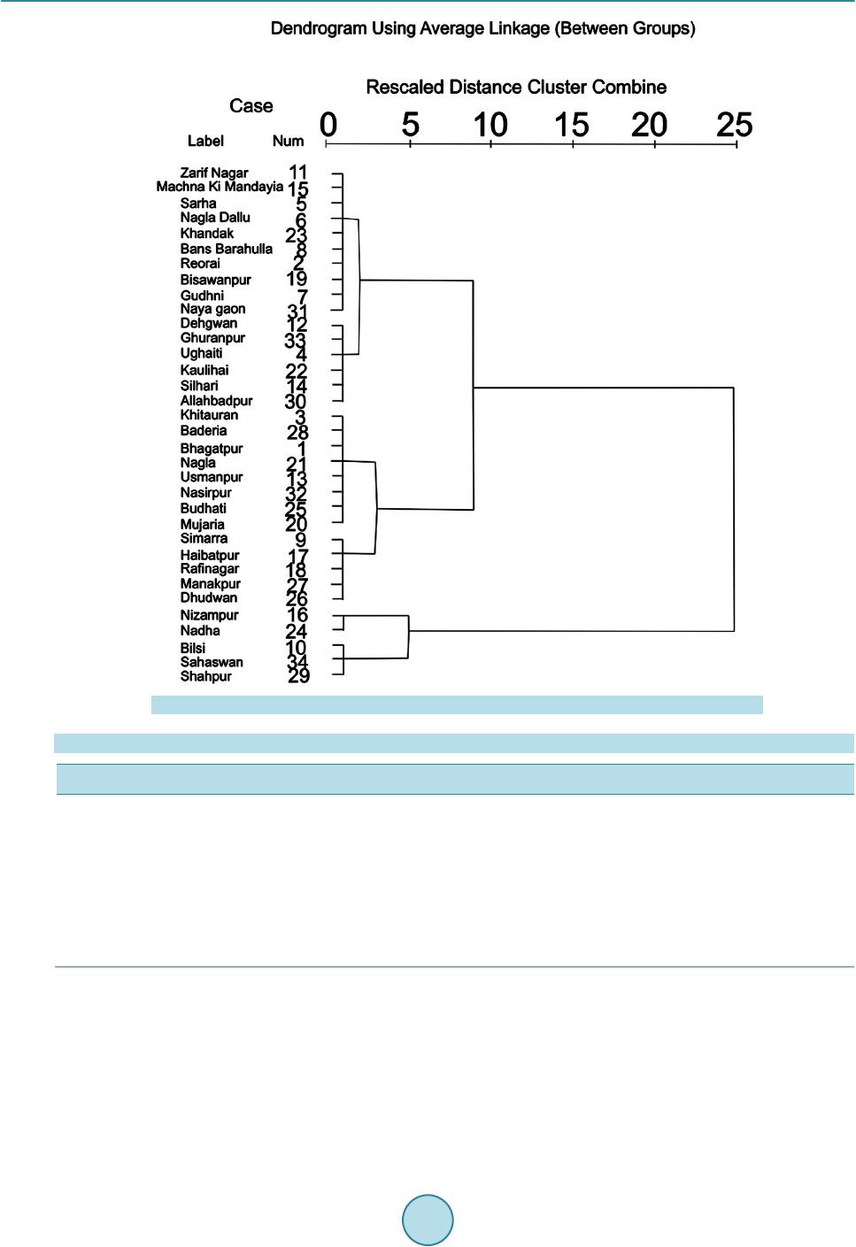

T. A. Khan
773
Figure 2. Dendrogram.
Table 1. Cluster groups and their members.
Group Members (Location/Sa mple No.)
A 11, 15, 5, 6, 23, 8, 2, 19, 7, 31
B 12, 33, 4, 22, 14, 30
C 3, 28, 1, 21, 13, 32, 25, 20
D 9, 17, 18, 27, 26
E 16, 24
F 10, 34, 29
The PCA of group B explains more than 95% of cumulative variance with HCO3 (0.991), Na (0.978) and K
(0.817) explaining the 33.686% of variance. The PCA of group of C explains cumulative variance of more than
82%. The EC, CO3 and Cl having the loading of 0.936, 0.918, and 0.911 respectively explains the total variance
of 40.071%.
The PCA of group D explains cumulative variance of more than 91%. The Cl and EC have the loading of
0.976 and 0.930, respectively, and explain the variance of 37.840%. The PC 2 of grou p D explains 32.073% of
variance and comprises of Mg, HCO3, and Na with loading of 0.954, 0.932 a nd 0.884, respe ctively. The P CA of

T. A. Khan
774
Table 2. Principal component analysis results for the five Clustering Groups stations.
Clustering Group Principal Component (PC) Principal Constituent Loading Proportion Variance (%)
A
PC1 Ca 0.805 25.025
CO3 0.898
PC2 HCO3 0.886 21.275
K 0.964
PC3 Na 0.852 21.236
Cl 0.819
PC4 pH 0.841 16.225
Ec 0.805
B
PC1
HCO3 0.991
33.686 Na 0.978
K 0.817
PC2 Cl 0.852 25.564
PC3 Mg 0.956 20.105
CO3 0.760
PC4 Ec 0.938 16.411
C
PC1
Ec 0.936
40.071 CO3 0.918
Cl 0.911
PC2 HCO3 0.933 22.542
PC3 Na 0.695 20.181
Cl 0.976
D
PC1 Ec 0.930 37.840
Mg 0.954
PC2
HCO3 0.932
32.073
Na 0.884
CO3 0.969
K 0.893
PC3 K 0.986 21.798
SO4 0.870
F
PC1
K 0.986
51.411
SO4 0.870
Cl 0.859
Na 0.858
PC2
CO3 0.986
48.589
HCO3 0.958
Na 0.858
Mg 0.738

T. A. Khan
775
group E only one component was extracted so, the solution cannot be rotated. The PCA of group F explains cu-
mulative variance of more than 100%. It extracts two components explaining variance of 51.411% and 48.589%.
The first component comprises of K (0.986) SO4 (0.870) and Cl (0.859), while the second component consist of
CO3 (0.986), HCO3 (0.958) Na (0.858) and Mg ( 0.738). The results of cluster and subsequent PC analysis show
some differences in compositio nal patterns of PCs, and water quality variables at dif ferent locations.
4.2. Overall Multivariate Characteristics of Groundwater Quality
In the present study ten variables are subjected to principal component analysis. Varimax rotation is used to
maximize the sum of the variance of the factor coefficients. The PCA of the hydrochemical data in parts of
Ganga-Sot s ub-basin (GSSB) extracted four Principal components of more than 1 eigen v alue with a cumulative
variance of 69.19% (Table 3). PCA I has eigenvalue of 2.093 and shows total variance of 20.926%. In this
component only
3
HCO
−
show strong positive loading (0.830), where as pH (−0.682) and
2
4
SO
−
(−0.659)
shows negative loading. The significantly high positive loading of
3
HCO
−
and high negative loading of pH is
suggestive of high supply CO2 and its subsequent mixing and conversion to
3
HCO
−
in the groundwater.
3
HCO
−
can form the fixation of CO2. For this purpose the CO2 is released by the dissolution of calcite and the
weathering of s ilicate minerals.
2
4
SO −
ions in the water are partly because of the dissolution of gypsum. Defi-
ciency of sulphate ions suggest water has more cations of Mg and Ca in the groundwater. High (negative) factor
loading of pH reflects the influence of acid-base factors on groundwater chemistry [39].
PCA II has an eigenvalue of 2.014. The data explains the variance of 20.136% with cumulative variance of
41.06%. It has two strongly correlated variables of Chloride and EC showing a strong positive loading of 0.92
and 0.814. High loading of these variables explains the geogenic influence on the quality of the groundwater.
Chloride remains stable once it enters a solution. High chloride content over to sodium may be due to base ex-
change process. Other source of it may be the leaching of saline residue from the soil.
PCA III with an eigenvalue 1.665 has a total variance of 16.65% and cumulative variance of 57.713%. This
factor shows moderate loading in the three variable potassium (0.68), sodium (0.663) and magnesium (0.521).
This factor is cation dominated. Mg2+ is a significant variable in this factor, which happens to be one of the ma-
jor ions in the hydrosphere and the most abundant divalent cation in the biosphere. It is an essential element for
both plants and animals [24]. A study in the Amazonian floodplain lake revealed that Ca2+, Mg2+ and Na+ sea-
sonality had been caused by abiotic processes while K+ evolution was controlled by aquatic macrophytes [40].
High loading of potassium and magnesium may be due to excessive use of synthetic fertilizers for agriculture
practices.
Table 3. Result of Principle component analysis of data of whole study area.
Component Matrixa
Chemical Variables 1 2 3 4
HCO3 0.830 −0.362 0.338 0.070
pH −0.682 −0.327 0.338 0.087
SO4 −0.659 −0.228 −0.045 0.252
Cl −0.041 0.920 0.089 −0.080
EC −0.028 0.814 0.292 0.125
K −0.005 −0.242 0.680 −0.053
Na 0.441 0.060 0.663 0.268
Mg 0.468 −0.267 −0.521 0.033
Ca −0.142 −0.105 0.043 0.811
CO3 0.263 0.263 −0.408 0.563
Eigenvalue 2.093 2.014 1.665 1.148
% of Variance 20.926 20.136 16.650 11.483
Cumulative % 20.926 41.062 57.713 69.196

T. A. Khan
776
The forth factor in analysis explains a total variance of 11.48% with an eigenvalue of 1.148. The factor ex-
plains the cumulative variance of 69.196%. The maximum loading is shown by Ca2+ (0.811) and
2
3
CO
−
(0.563).
The availability Calcium in groundw ater is due to the presence of soluble calcium-containing solids and of sul-
fur in the form of sulphate.
4.3. Test of Hypothesis
The PCA for the variables falling exclusively in the region of clayey loam soil/Ganga-Mahwa lowland resulted
in five PCs (Table 4) which explain 91% of variance in the data set. In the analysis only components with eigen-
value more than one are taken into consideration. The first component explains 29.923% of variance. The first
component has EC, CO3, HCO3, Cl and Na with positive loading and pH and SO4 with high negative loading
This component can be termed as an anion component and shows.
The second component explains 24.24% of variance with high positive loading in HCO3 (0.703), K (0.706)
and Mg (0.627) and negative loading of 0.646 of Cl. The third component explains 14.78% of variance and
gives positive loading in Ca (0.702) and Mg (0.621). The fourth and fifth components have one variable each
explaining the variance of 12.52% and 10.17% respectively. The fourth component consist of CO3 with negative
loading o f 0.647 and fifth component ex pl a i ning 10.17% of variance wit h Na ha ving loading of 0. 60 8.
The first four factors for the sandy soil /Central-Upland explain 80% of the variance (Table 5 ). The first prin-
cipal component explains around 26% of variance. The EC, Cl, K, Mg gives a moderate positive loading while
pH shows a strong negative loading. This component can be taken as a salinity controlled component. The mean
value of EC of the samples in sandy soil region is around 576 micromhos/cm which is more than that of clayey
loam and less than of loam soil type region. Range of EC in the groundwater of central-upland is 240 - 1039 mi-
cromhos/cm. The second principal component explains around 24% of variance. HCO3, Cl and Mg gives a h igh
negative loading while SO4 gives a moderate positive loading. The third principal component extracts EC and
Na with moderate positive loading and explains around 15% of total variance. The fourth principal component
comprises of CO3 and Na with positive loading explains around 13% of total variance in data.
Table 4. Showing only cases fo r which clay ey loam type soil are used in the analysis phase.
Component Matrix
Component
1 2 3 4 5
pH −0.702 −0.379 −0.114 0.430 0.337
Ec 0.715 −0.461 0.007 0.288 0.226
CO3 0.520 −0.332 −0.289 −0.647 0.124
HCO3 0.668 0.703 0.019 0.009 0.158
Cl 0.557 −0.646 −0.270 0.344 −0.072
SO4 −0.742 0.078 0.334 −0.211 0.434
Na 0.589 0.166 0.481 −0.047 0.608
K 0.230 0.706 0.292 0.487 −0.257
Ca 0.071 −0.351 0.702 −0.337 −0.426
Mg −0.080 0.627 −0.621 −0.225 0.020
Eigenvalue 2.992 2.424 1.477 1.253 1.017
% of Variance 29.923 24.244 14.766 12.525 10.170
Cumulative % 29.923 54.167 68.933 81.458 91.628

T. A. Khan
777
Table 5. Showing only cases for which sandy type of soil are used in the analysis phase.
Component Matrix
Component
1 2 3 4
pH −0.851 0.321 −0.028 −0.061
Ec 0.632 0.335 0.662 −0.133
CO3 0.441 0.182 −0.148 0.671
HCO3 −0.205 −0.875 0.323 0.187
Cl 0.625 0.600 0.417 −0.004
SO4 −0.208 0.631 −0.329 0.483
Na −0.301 −0.290 0.642 0.551
K −0.654 0.342 0.402 0.285
Ca 0.000 −0.435 0.191 −0.225
Mg 0.549 −0.556 −0.334 0.418
Eigenvalue 2.614 2.471 1.570 1.350
% of Variance 26.144 24.709 15.699 13.501
Cumulative % 26.144 50.852 66.551 80.053
The PCA of variables falling on the loam type of soil /Sot plain extracts three PC’s (Table 6) explaining a
cumulative variance of 91.751%. The first component explains around 43% of variance and a high eigenvalue of
4.389. All the extracted variables i.e. pH, EC, and SO4 gives strong positive loading and HCO3 and K shows a
strong negative loading. The second principal component also shows a strong loading and extracts Cl, and Na
with a strong negative loading and Mg with a strong negative loading. The third principal component extracts
CO3 and Ca with strong loading and SO4 and K with a weak positive loading. The mean EC in the loam type of
soil is highest among the three types i.e. 602.2 micromhos/cm.
4. Discussion
The PCA of the whole basin extracts five principal components explaining a cumulative variance of 69.196%
while the PCA of sub-divided area results show: clayey loam-five PCs with 91.628% cumulative variance,
sandy soil-four PCs with 80.053% of cumulative variance, loam type of soil-three PCs with 91.754% of variance.
So the data set is well characterized with sub-divisions. The three soil types show different valid result.
The Ganga-Mahawa sub region where the top soil is loam to clayey loam is the flood plain area of River
Ganga and Mahawa. The pH and SO4 concentration in the groundwater has high negative loading and has an in-
verse relation the EC and HCO3.
The Central-upland sub regions is marked by sandy soil with poor drainage. In local parley this area is re-
ferred as “Bhur” has thick aquifers which manifest the channel deposit. The PCA for the groundwater samples
of this sub-region extracted four components, explaining the cumulative variance of 80.053%. The pH has high
negative loading >8 and has inver se relation with EC, Cl and Mg.
The pH in two sub regions gives a high negative loading and in one region that is in Sot upland it has a high
positive loading. This is also reflected in the PCA results of the whole area where pH loading is negative. The
negative loading of pH in three sub-divisions explains the aggressiveness of acidic media towards th e soil which
in return increases the concentration of other variables. This can be said that the PCA result pattern varies when
the area is sub divided but the dominant component is reflected in the combined analysis. Over loading of EC is
insignificant but in analysis of sub-divided region the EC loading varies from 0.632 to 0.959. Medium to high
loading o f EC is not reflected in the combined PCA.

T. A. Khan
778
Table 6. Showing only cases for which loam type of soil are used in the analysis phase.
Component Matrix
Components
1 2 3
pH 0.820 0.431 0.030
EC 0.959 −0.048 −0.186
CO −0.218 0.340 0.905
HCO3 −0.806 0.294 0.102
Cl 0.296 −0.841 −0.330
CO4 0.846 0.150 0.510
Na −0.355 −0.865 −0.059
K 0.820 −0.076 0.552
Ca 0.250 0.258 0.897
Mg −0.087 0.911 0.307
Eigenvalue 4.389 3.475 1.311
% of variance 43.885 34.754 13.111
Cumulative % 43.885 78.639 91.751
5. Conclusion
The PCA of sub divided region shows a good cumulative variation than that of whole area data analysis. This
suggests that the groundwater pattern of the three distinct physiographic regions is different. And each physio-
graphic region has a different groundwater quality as manifested in PCA. PCA can not only be used for data re-
duction purposes but safely be used for the characterisation of groundwater chemistry. The vadose zone geo-
chemistry was not done in the area therefore it cannot safely be said that there is influence of top soil on the
groundwater. But one thing is clear that the groundwater chemistry pattern is different in aquifers falling below
distinct physiographic regions.
Acknowledgements
The author is thankful to the Chairman Department of Geology for providing necessary facilities needed to carry
out the present work .
References
[1] Khan, T.A. (2014) An Overview of Cli mate Change and Groundwater Status in Parts of Central Ganga Plain. Journal
of Engineering Computers & Applied Sciences, 3, 1-5.
[2] Nigam, A., Gujia, B. and Bandyopadhya, J. (1998) Fresh Water for India’s Children and Nature. UNICEF-WWF, New
Delhi.
[3] Samadder, R.K., Kumar, S. and Gupta, R.P. (2011) Paleochannels and Their Potential for Artificial Groundwater Re-
charge in the Western Ganga Plains. J ournal of Hydrology, 400, 154-164.
http://dx.doi.org/10.1016/j.jhydrol.2011.01.039
[4] Das, D., Samanta, G., Mandal, B.K., Chowdhury, T.R., Chanda, C.R., Chowdhury, P.P., Basu, G.K. and Chakraborti,
D. (1996) Arsenic in Groundwater in Six Districts of West Bengal, India. Environmental Geochemistry and Health, 18,
5-15 http://dx.doi.org/10.1007/BF01757214
[5] Singh, K.P., Malik, A., Singh, V.K., Mohan, D. and Sinha, S. (2005) Chemometric Analysis of Groundwater Quality
Data of Alluvial Aquifer of Gangetic Plain, North India. Analytica Chimica Acta, 550, 82-91.
http://dx.doi.org/10.1016/j.aca.2005.06.056

T. A. Khan
779
[6] Ayoko, G.A., Singh, K., Balerea, S. and Kokot, S. (2007) Exploratory Multivariate Modeling and Prediction of the
Phys ico-Chemical Properties of Surface Water and Groundwater. Journal of Hydrology, 336, 115-124.
http://dx.doi.org/10.1016/j.jhydrol.2006.12.013
[7] Qian, Y., Migliaccio, K.W., Wan, Y. and Li, Y. (2007) Surface Water Quality Evaluation Using Multivariate Methods
and a New Water Quality Inde x in the Indian River Lagoon, Florida. Water Resources Research, 43.
[8] Seyhan, E., van-de-Griend, A.A. and Engelen, G.B. (1985) Multivariate Analysis and Interpretation of the Hydro-
chemistry of a Dolomitic Reef Aquifer, Northern Italy. Water Resources Research, 21, 1010-1024.
http://dx.doi.org/10.1029/WR021i007p01010
[9] Reeve, A.S., Siege l, D.I. and Glaser, P.H. (1996) Geochemical Controls on Peatland Pore Water from the Hudson Bay
Lowland: A Multivariate Statistical Approach. Journal of Hydrology, 181, 285-304.
http://dx.doi.org/10.1016/0022-1694(95)02900-1
[10] Ochsenkuehn, K.M., Kontoyannakos, J. and Ochsenkuehn, P.M. (1997) A New Approach to a Hydrochemical Study of
Ground Water Flow. Journal of Hydrology, 194, 64-75. http://dx.doi.org/10.1016/S0022-1694(96)03218-0
[11] Meng, S.X. and Maynard, J.B. (2001) Use of Statistical Analysis to Formulate Conceptual Models of Geochemical
Behavior: Water Chemical Data from the Botucatu Aquifer in Sao Paulo State, Brazil. Journal of Hydrology, 250, 7 8-
97. http://dx.doi.org/10.1016/S0022-1694(01)00423-1
[12] Danielsson, A., Cato, I., Carman, R. and Rahm, L. (1999) Spatial Clustering of Metals in the Sediments of the Skager-
rak/Kattegat. Applied Geochemistry, 14, 689-706. http://dx.doi.org/10.1016/S0883-2927(99)00003-7
[13] Chen, K., Jiao, J.J., Huang, J. and Huang, R. (2007) Multivariate Statistical Evaluation of Trace Elements in Ground-
water in a Coastal Area in Shenzhen, China. Environmental Pollution, 147, 771-780.
http://dx.doi.org/10.1016/j.envpol.2006.09.002
[14] Khan, T.A. (2008) Cluster Analysis and Quality Assessment of Groundwater in and around Aligarh City, U.P. India.
Proceedings of All India Seminar on Advances in Environmental Science and Technology, Zakir Hussain College of
Engineering and Technology, A.M.U, Aligarh, 15-16 February 2008, 109-114.
[15] Bollen, K.A. (1989) Structural Equations with Latent Variables. John Wiley & Sons, New York, 528 p.
http://dx.doi.org/10.1002/9781118619179
[16] Park, H.S., Dailey, R. and Lemus, D. (2002) The Use of Principal Factor Analysis and Principal Components Analysis
in Communication Research. Human Communication Research, 28, 562-577.
http://dx.doi.org/10.1111/j.1468-2958.2002.tb00824.x
[17] Bengraine, K. and Marhaba, T.F. (2003) Using Principal Component Analysis to Monitor Spatial and Temporal
Changes in Water Quality. Journal of Hazardous Materials, 100, 179-195.
http://dx.doi.org/10.1016/S0304-3894(03)00104-3
[18] Wold, S., E sbe nsen, K. and Geladi , P. (1987) Principal Component Analysis. Chemometrics and Intelligent Laboratory
Systems, 2, 37-52. http://dx.doi.org/10.1016/0169-7439(87)80084-9
[19] Farnham, I.M., Johannesson, K.H., Singh, A.K., Hodge, V.F. and Stetzenbach, K.J. (2003) Factor Analytical Ap-
proaches for Evaluating Groundwater Trace Element Chemistry Data. Analytica Chimica Acta, 490, 123-138.
http://dx.doi.org/10.1016/S0003-2670(03)00350-7
[20] Andrade, E.M., Palácio, H.A.Q., Crisóstomo, L.A., Souza, I.H. and Teixeira, A.S. (2005) Índice de qualidade de água,
uma proposta para o vale do rio Trussu. Ceará. Revista Ciencia Agronómica, 36, 135-142. (in Portuguese)
[21] Mazlum, N., Ozer, A. and Mazlum, S. (1999) Interpretation of Water Quality Data by Principal Component Analysis.
Journal of Engineering and Environmental Science, 23, 19-26.
[22] Aiuppa, A., Bellomo, S., Brusca, L., D’Alessandro, W. and Federico, C. (2003) Natural and Anthropogenic Factors
Affecting Groundwater Quality of an Active Volcano (Mt. Etna, Italy). Applied Geochemi st ry , 18, 863-882.
http://dx.doi.org/10.1016/S0883-2927(02)00182-8
[23] Mandal, U.K., Warrington, D.N., Bhardwaj, A.K., Bar-Tal, A., Kautsky, L., Minz, D. and Levy, G.J. (2007) Evaluating
Impact of Irrigation Water Quality on a Calcareous Clay Soil Using Principal Component Analysis. Geo derma , 144,
189-197. http://dx.doi.org/10.1016/j.geoderma.2007.11.014
[24] Khan, T.A. (2011) Multivarite Analysis of Hydrochemical Data of the Groundwater in Parts of Karwan Sengar Sub
Basin, Central Ganga Basin. Glo bal NEST Journal, 13, 229-236.
[25] Yu, Y.S. and Zou, S. (1993) Relating Trends of Principal Components to Trends of Water-Quality Constituents.
JAWRA Journal of the American Water Resources Association, 29, 797-806.
http://dx.doi.org/10.1111/j.1752-1688.1993.tb03239.x
[26] Antonietti, R. and Sartore, F. (1996) Optimization of Parameters Used for Freshwater Survey. Water Research, 30,
1535-1538. http://dx.doi.org/10.1016/0043-1354(95)00299-5

T. A. Khan
780
[27] Reisenhofer, E., Adami, G. and Barbieri, P. (1998) Using Chemical and Physical Parameters to Define the Quality of
Karstic Freshwaters (Timavo River North-Eastern Italy ): A Chemometric Approach. Water Resea rch, 32, 1193-1203.
http://dx.doi.org/10.1016/S0043-1354(97)00325-4
[28] Camdevyren, H., Demyr, N., Kanik, A. and Keskyn, S. (2005) Use of Principal Component Scores in Multiple Linear
Regression Models for Prediction of Chlorophyll-a in Reservoirs. Ecological Modelling, 181, 581-589.
http://dx.doi.org/10.1016/j.ecolmodel.2004.06.043
[29] Ouyang, Y. (2005) Evaluation of River Water Quality Monitoring Stations by Principal Component Analysis. Water
Research, 39, 2621-2635. http://dx.doi.org/10.1016/j.watres.2005.04.024
[30] Kowalkowski, T., Z bytniewski , R., Szpejna, J. and Buszewski, B. (2006) Application of Chemometrics in River Water
Classification. Water Research, 40, 744-752. http://dx.doi.org/10.1016/j.watres.2005.11.042
[31] Singh, I. B. (1996) Geological Evolution of Ganga Plain—An Overview. Journal of the Palaeontological Society of In-
dia, 41, 99-137.
[32] Shukla, U.K. and Bora, D.S. (2003) Geomorphology and Sedimentology of Piedmont Zone, Ganga Plain, India. Cur-
rent Science, 84, 1034-1040.
[33] Tandon, S.K., Gibling, M.R., Sinha, R., Singh, V., Ghazanfari, P., Dasgupta, A., Jain, M. and Jain, V. (2006) Alluvial
Valleys of the Ganga Plain, India; Timing and Causes of Incision. Special Publication—Society for Sedimentary Ge-
ology, 85, 15-35.
[34] Shukla, U.K. and Raju, N.J. (2008) Migration of the Ganga River and Its Implication on Hydro-Geological Potential of
Varanasi Area, U.P., India. Journal of Earth System Science, 117, 489-498.
http://dx.doi.org/10.1007/s12040-008-0048-4
[35] Oldham, R.D. (1917) On Probable Changes in the Geography of the Punjab and Its Rivers—An Historico-Geographi-
cal Study. Journal of the Asiatic Society of Bengal, 55, 322-343.
[36] Garcia-Hernan, O., Sahun, O., Perez, P. and Suso, J.M. (1988) Estudio de contaminacion de aguas subterraneas en la
zona industrial norte de Valladolid Proceedings of Second Congresso Geologico de Espana, Vol. 2, Granada, Spain,
399.
[37] APHA (1989) Standard Methods for Examination of Water and Wastewater. 17th Edition, American Public Health
Association, Washington DC.
[38] Liu, C.W., Li n, K.H. and Kuo, Y.M. (2003) Application of Factor Analysis in the Assessment of Groundwater Quality
in a Blackfoot Disease Area in Taiwan. Science of the Total Environment, 313, 77-89.
http://dx.doi.org/10.1016/S0048-9697(02)00683-6
[39] Dragon, K. (2003) The Chemistry of the Wielkopolska Buried Valley Aquifer (Region between Obra and Warta rivers).
PhD Thesis, Adam Mickiewicz University, Poznan. (In Polish)
[40] Weber, G.E., Furch, K. and Junk, W.J. (1996) A Simple Modelling Approach towards Hydrochemical Seasonality of
Major Cations in a Central Amazonian Floodplain Lake. Ecological Modelling, 91, 39-56.
http://dx.doi.org/10.1016/0304-3800(95)00165-4