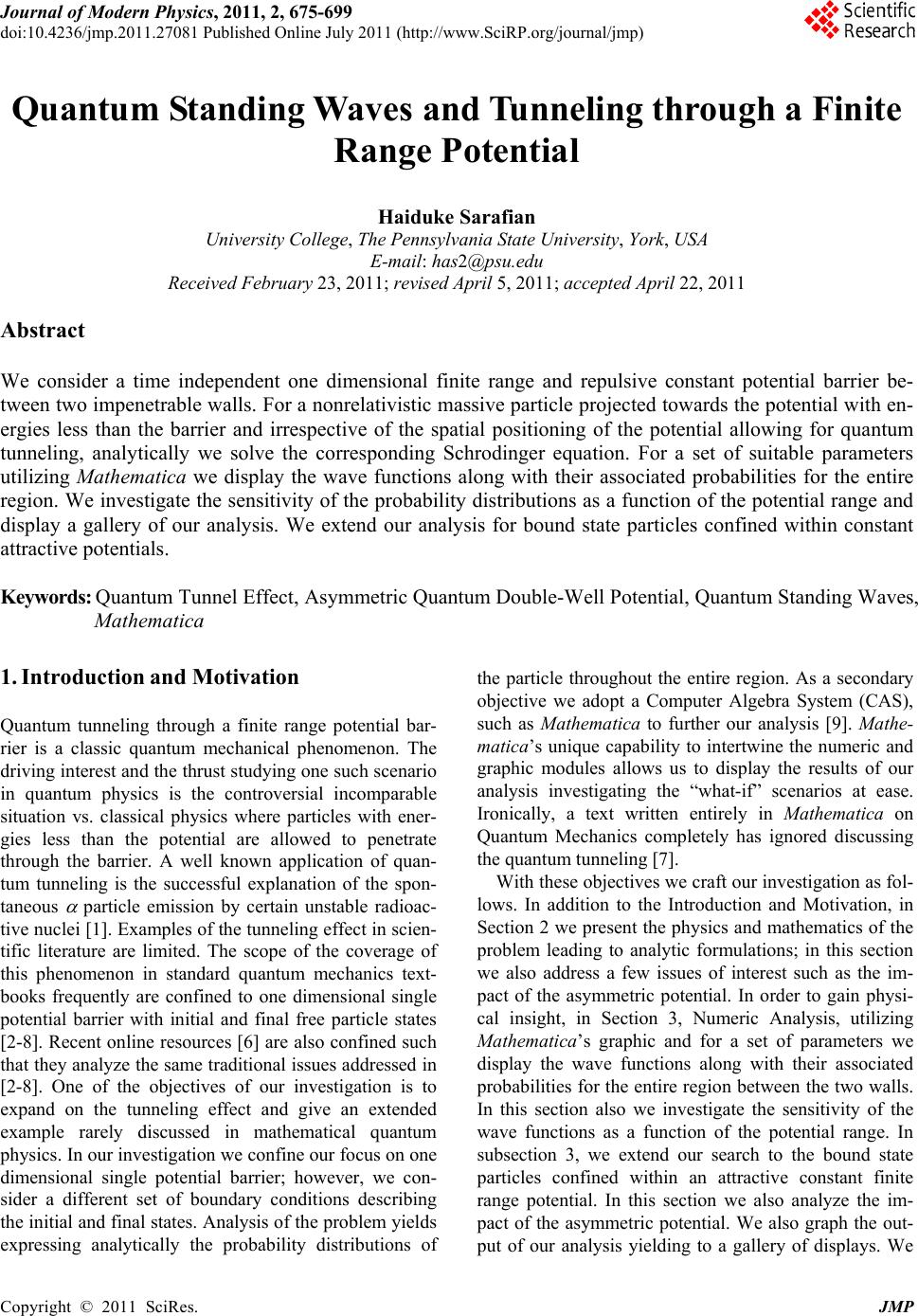
Journal of Modern Physics, 2011, 2, 675-699
doi:10.4236/jmp.2011.27081 Published Online July 2011 (http://www.SciRP.org/journal/jmp)
Quantum Standing Waves and Tunneling through a Finite
Range Potential
Haiduke Sarafian
University College, The Pennsylvania State University, York, USA
Received February 23, 2011; revised April 5, 2011; accepted April 22, 2011
Abstract
We consider a time independent one dimensional finite range and repulsive constant potential barrier be-
tween two impenetrable walls. For a nonrelativistic massive particle projected towards the potential with en-
ergies less than the barrier and irrespective of the spatial positioning of the potential allowing for quantum
tunneling, analytically we solve the corresponding Schrodinger equation. For a set of suitable parameters
utilizing Mathematica we display the wave functions along with their associated probabilities for the entire
region. We investigate the sensitivity of the probability distributions as a function of the potential range and
display a gallery of our analysis. We extend our analysis for bound state particles confined within constant
attractive potentials.
Keywords: Quantum Tunnel Effect, Asymmetric Quantum Double-Well Potential, Quantum Standing Waves,
Mathematica
1. Introduction and Motivation
Quantum tunneling through a finite range potential bar-
rier is a classic quantum mechanical phenomenon. The
driving interest and the thrust studying one such scenario
in quantum physics is the controversial incomparable
situation vs. classical physics where particles with ener-
gies less than the potential are allowed to penetrate
through the barrier. A well known application of quan-
tum tunneling is the successful explanation of the spon-
taneous
 particle emission by certain unstable radioac-
tive nuclei [1]. Examples of the tunneling effect in scien-
tific literature are limited. The scope of the coverage of
this phenomenon in standard quantum mechanics text-
books frequently are confined to one dimensional single
potential barrier with initial and final free particle states
[2-8]. Recent online resources [6] are also confined such
that they analyze the same traditional issues addressed in
[2-8]. One of the objectives of our investigation is to
expand on the tunneling effect and give an extended
example rarely discussed in mathematical quantum
physics. In our investigation we confine our focus on one
dimensional single potential barrier; however, we con-
sider a different set of boundary conditions describing
the initial and final states. Analysis of the problem yields
expressing analytically the probability distributions of
the particle throughout the entire region. As a secondary
objective we adopt a Computer Algebra System (CAS),
such as Mathematica to further our analysis [9]. Mathe-
matica’s unique capability to intertwine the numeric and
graphic modules allows us to display the results of our
analysis investigating the “what-if” scenarios at ease.
Ironically, a text written entirely in Mathematica on
Quantum Mechanics completely has ignored discussing
the quantum tunneling [7].
With these objectives we craft our investigation as fol-
lows. In addition to the Introduction and Motivation, in
Section 2 we present the physics and mathematics of the
problem leading to analytic formulations; in this section
we also address a few issues of interest such as the im-
pact of the asymmetric potential. In order to gain physi-
cal insight, in Section 3, Numeric Analysis, utilizing
Mathematica’s graphic and for a set of parameters we
display the wave functions along with their associated
probabilities for the entire region between the two walls.
In this section also we investigate the sensitivity of the
wave functions as a function of the potential range. In
subsection 3, we extend our search to the bound state
particles confined within an attractive constant finite
range potential. In this section we also analyze the im-
pact of the asymmetric potential. We also graph the out-
put of our analysis yielding to a gallery of displays. We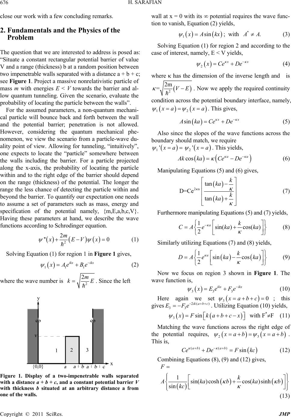

H. SARAFIAN 676
wall at x = 0 with its  potential requires the wave func-
tion to vanish, Equation (2) yields,
close our work with a few concluding remarks.
2. Fundamentals and the Physics of the
Problem
The question that we are interested to address is posed as:
“Situate a constant rectangular potential barrier of value
V and a range (thickness) b at a random position between
two impenetrable walls separated with a distance a + b + c;
see Figure 1. Project a massive nonrelativistic particle of
mass m with energies E < V towards the barrier and al-
low quantum tunneling. Given the scenario, evaluate the
probability of locating the particle between the walls”.
For the assumed parameters, a non-quantum mechani-
cal particle will bounce back and forth between the wall
and the potential barrier; penetration is not allowed.
However, considering the quantum mechanical phe-
nomenon, we view the scenario from a particle-wave du-
ality point of view. Allowing for tunneling, “intuitively”,
one expects to locate the “particle” somewhere between
the walls including the barrier. For a particle projected
along the x-axis, the probability of locating the particle
within and to the right edge of the barrier should depend
on the range (thickness) of the potential. The longer the
range the less chance of detecting the particle within and
beyond the barrier. To quantify our expectation one needs
to assume a set of parameters such as mass, energy and
specification of the potential namely, {m,E,a,b,c,V}.
Having these parameters at hand, we describe the wave
functions according to Schrodinger equation.




1sin
x
Akx  ; with *.
A
A (3)
Solving Equation (1) for region 2 and according to the
case of interest, namely, E < V yields,


2
x
x
x
Ce De





(4)
where  has the dimension of the inverse length and is

2
2m
=VE  
. Now we apply the required continuity
condition across the potential boundary interface, namely,




12
x
ax  a

. This gives,


sin
x
x
A
ka CeDe

 
 (5)
Also since the slopes of the wave functions across the
boundary should match, we require


1'
x
a 




2'
x
a 

. This yields,




cos a AkkaCe De




a
(6)
Manipulating Equations (5) and (6) gives,


2a
tan
D=Ce
tan
k
ka
k
ka














(7)
Furthermore manipulating Equations (5) and (7) yields,
1sin( )cos( )
2
ak
CA ekaka















(8)
 
2
2
'' 0
m
xEVx   
 (1) Similarly utilizing Equations (7) and (8) yields,
 
1sin cos
2
ak
DA ekaka














Solving Equation (1) for region 1 in Figure 1 gives, (9)

111
ikx ikx
x
Ae Be 

 (2)
Now we focus on region 3 shown in Figure 1. The
wave function is,
2
2m
kE
where the wave number is . Since the left


333
ikx ikx
x
Ee Fe 

 (10)
Here again we set; this
gives

30x abc
  

2( )
33
ik abc
EFe


 . Utilizing Equation (10) yields,




3sin
x
F kabcx  



 with F*F (11)
Matching the wave functions across the right edge of
the potential requires,

23
x
abx ab   .
This is,

()() sin ab ab
CeDeF kc
 
 (12)
Combining Equations (8), (9) and (12) gives,
  
1sin( )coshcos( )sinh
sin
F
k
Akabka
kc


b

















Figure 1. Display of a two-impenetrable walls separated
with a distance a + b + c, and a constant potential barrier V
with thickness b situated at an arbitrary distance a from
one of the walls.
(13)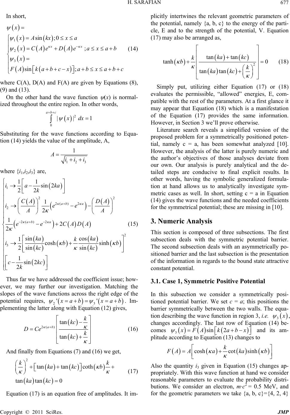

H. SARAFIAN677
In short,

 
 

 
1
2
3
sin ;0
;
sin ;
xx
x
xA kxxa
x
CAeDAeaxa b
x
F
Akabcxabxabc







 
 







(14)
where C(A), D(A) and F(A) are given by Equations (8),
(9) and (13).
On the other hand the wave function
 (x) is normal-
ized throughout the entire region. In other words,

2
0
||
abc
xdx 


1
Substituting for the wave functions according to Equa-
tion (14) yields the value of the amplitude, A,
123
1
Aiii 
where {i1,i2,i3} are,





 

    

1
2
2( )2
2
2( )2
2
3
11
sin2
22
1
2
12
2
sin cos
1cosh sinh
2sin sin
1sin 2
2
ab a
ab a
ia ka
k
CA DA
iee
A
eeCADA
ka ka
k
ib
kc kc
ckc
k







 





 

 
 














2
A
b 




(15)
Thus far we have addressed the coefficient issue; how-
ever, we may further our investigation. Matching the
slopes of the wave functions across the right edge of the
potential requires,

23
''
x
abx ab   . Im-
plementing the latter along with Equation (12) gives,


2()
tan
tan
ab
k
kc
DCe k
kc











(16)
And finally from Equations (7) and (16) we get,
 
 
2
tantan coth
tan tan0
k
ka kcb
ka kc




 


k


(17)
Equation (17) is an equation free of amplitudes. It im-
plicitly intertwines the relevant geometric parameters of
the potential, namely {a, b, c} to the energy of the parti-
cle, E and to the strength of the potential, V. Equation
(17) may also be arranged as,
  
 
2
tantan
tanh 0
tan tan
ka kc
k
b
k
ka kc















(18)
Simply put, utilizing either Equation (17) or (18)
evaluates the permissible, “allowed” energies, E, com-
patible with the rest of the parameters. At a first glance it
may appear that Equation (18) which is a manifestation
of the Equation (17) provides the same information.
However, in Section 3 we’ll prove otherwise.
Literature search reveals a simplified version of the
proposed problem for a symmetrically positioned poten-
tial, namely c = a, has been somewhat analyzed [10].
However, the analysis of the latter is purely numeric and
the author’s objectives of those analyses deviate from
our own. Our analysis is purely analytical and the de-
tailed steps are conducive to final explicit results. In
other words, having the symbolic generalized formula-
tion at hand allows us to analytically investigate sym-
metric cases as well. In short, setting c = a in Equation
(14) gives the wave functions and the needed coefficients
for the symmetrical potential; these are missing in [10].
3. Numeric Analysis
This section is composed of three subsections. The first
subsection deals with the symmetric potential barrier.
The second subsection deals with an asymmetrically po-
sitioned barrier and the last subsection is the presentation
of the information in regards to the bound state attractive
constant potential.
3.1. Case 1, Symmetric Positive Potential
In this subsection we consider a symmetrically posi-
tioned potential barrier. We set c = a; this positions the
barrier symmetrically between the two walls. The equa-
tion describing the wave function in region 3, i.e.


3
x
 ,
changes accordingly. The last row of Equation (14) be-
comes




3sin 2

x
FAka b x  



 and its am-
plitude according to Equation (13) changes to
  
coshcot sinh
k
F
AAaka b 








Also the quantity i3 given in Equation (15) changes ap-
propriately. With this wave function at hand we consider
reasonable parameters to evaluate the probability distri-
butions. We consider an electron, m·c2 = 0.5 MeV, and
for the geometric parameters we take {a, b, c}={4, 2, 4}

H. SARAFIAN 678
angstrom, and we set V = 10 eV. Substituting for 197c


Mev fm, the wave number k and the quantity
 in the
units of 1/Å become,


22
100. 100.
,2,2
0.50764 ,0.50764
kmcEmcV
cc
EVE


 E



 
In these quantities the energy, E, is to be entered in eV
units.
The chosen set of parameters is intertwined via either
Equation (17) or Equation (18). To evaluate the permis-
sible values of energy E one may graph the left hand side
of Equation (18) and hunt for compatible energies within
the range 0 < E < V. Alternatively one may plot Equation
(17) and look for its intersecting coordinates with the E
axis. Equation (18), however, is a second order algebraic
equation with two distinct roots. Therefore, we solve
Equation (17) and plot functions associated with its roots
along with the plot of the left hand side of Equation (18).
This gives two separate graphs shown in Figure 2.
This analysis is critical for appropriately grouping the
roots of the equations. Without this analysis one may
apply the unsorted roots of Equation (18) achieving un-
sightly conclusions. Overlaid plots of Equation (18)
along with the plots of the root equations of Equation (17)
provide the natural sorting. The red curve of top graph of
Figure 2 is the positive root of Equation (17) while the
green curve is the plot of Equation (18). This clearly
shows the red curve intersects with the smaller values of
the paired green intercepts. On the contrary, as shown on
the bottom graph the plot of the other root of Equation
(17) intersects at the larger values of the paired green
intercepts. In short, with this learned insight one would
be better off seeking the roots of Equation (17) sepa-
rately rather than seeking the roots of Equation (18). Al-
ternatively, if one chooses to utilize Equation (18) one
would need to be cautious sorting the roots conducive the
same previous conclusions. Having said all this, now we
pursue evaluating the sorted roots of Equation (17).
These are tabulated in Table 1.
In Table 1, the first row, “Plus”, corresponds to the
positive roots of Equation (17), and the second row,
“Minus”, is the corresponding roots of the negative root
equation. With these values of permissible energies we
plot the wave functions and their associated probability
distributions; these are shown in Figure 3. There are two
permissible energies; their ordered list is n = {1, 2}. It is
notable that the lower energies of each set are associated
with the even wave functions. These are the first plots of
graphs of each row. The wave functions are symmetrical
about the center of the potential barrier. For a visual un-
derstanding three different colors are used to show the
wave functions in different regions. The continuity of the
2 4 6810
2.0
EeV
0.5
1.0
1.5
2 4 6 810
E
eV
2
.0
EeV
0.5
1.0
1.5
E
eV
Figure 2. The green curve is the plot of left hand side of
Equation (18). The red curve on the left graph is the plot of
the positive root of Equation (17), while the blue curve of
the right plot is the display of the negative root of Equation
(17).
Table 1. The entries in the first row are the roots of Equa-
tion (17) associated with its positive root. The second row is
the repeat of the same scenario for the negative roots.
Root 1 Root 2
Plus 1.72966 6.56287
Minus1.82285 7.19653
wave functions across the edges of the potential barrier
clearly is depicted. The wave functions associated with
the higher permissible energy set are depicted in the
middle column. These wave functions are asymmetric
and three different colors are used to show the associated
wave functions in their respective regions. The author is
pleased to point out that color coding concept of the re-
gional wave functions is novel and unique to this project.
As required the wave functions are clamped at both
ends. The lowest permissible energy is associated with
the simplest configuration of the even wave function and
is represented by the top graph. The latter wave function
is a symmetrical function with respect to the center of the
potential barrier and it does not cross the horizontal axis.
On the contrary, the energy of the odd wave function is
higher than the corresponding even wave function and it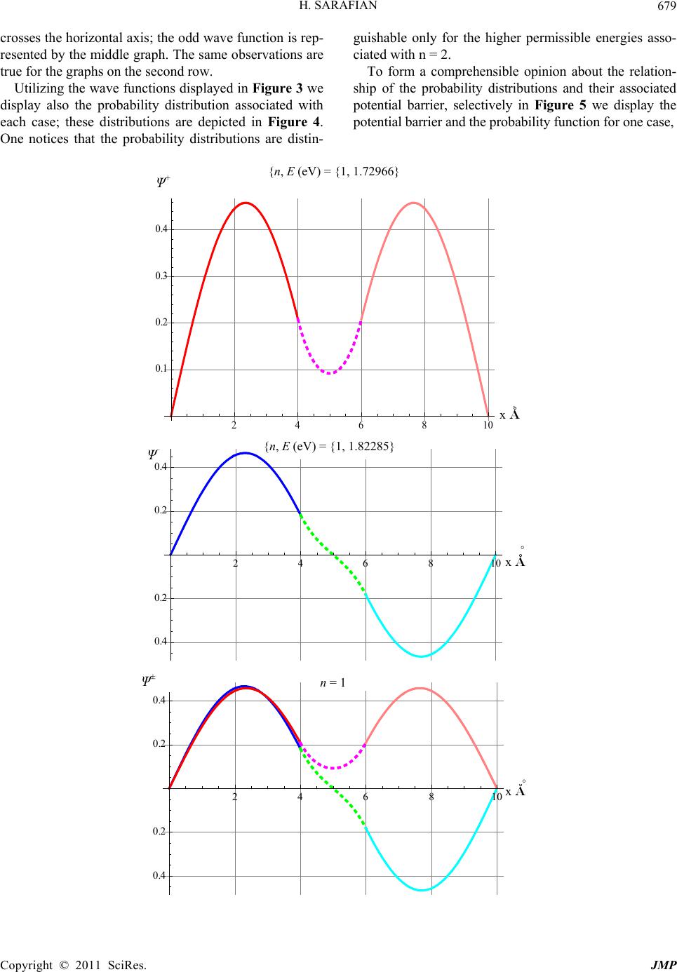

H. SARAFIAN 679
crosses the horizontal axis; the odd wave function is rep-
resented by the middle graph. The same observations are
true for the graphs on the second row.
Utilizing the wave functions displayed in Figure 3 we
display also the probability distribution associated with
each case; these distributions are depicted in Figure 4.
One notices that the probability distributions are distin-
guishable only for the higher permissible energies asso-
ciated with n = 2.
To form a comprehensible opinion about the relation-
ship of the probability distributions and their associated
potential barrier, selectively in Figure 5 we display the
potential barrier and the probability function for one case,
2
468 10
n
,
E
eV 1, 1.72966
{n, E (eV) = {1, 1.72966}
Ψ+
x A
°
0.1
0.2
0.3
0.4
x
Å
2
4
68 10
{n, E (eV) = {1, 1.82285}
x A
°
0.4
0.2
0.2
0.4
Ψ
-
x
Å
n = 1
2
4
68 1
0
x A
°
0.4
0.2
0.2
Ψ±
0.4
x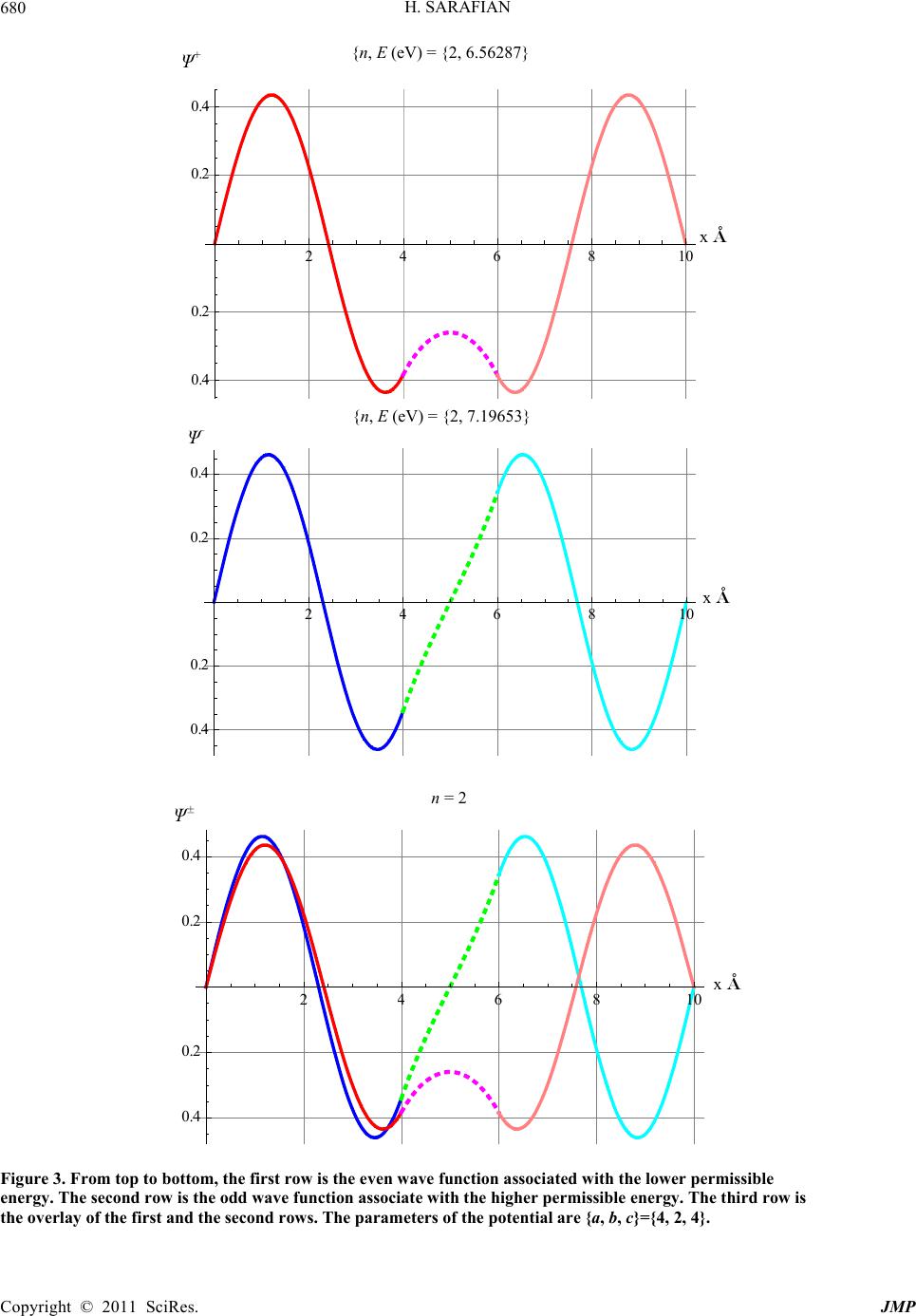
Å

H. SARAFIAN 680
2
4
68 1
0
n
,
E
eV
2
, 6.56287
{n, E (eV) = {2, 6.56287}
x A
°
0.4
0.2
0.2
0.4
Ψ+
x
Å
n
,
E
eV
2
, .196537
{n, = {2 7 E (eV),.19653}
2
4
6810 x
A
°
0.4
0.2
0.2
0.4
Ψ-
x
Å
2
4
68 1
0
n
2
n = 2
Ψ±
x A
°
0.4
0.2
0.2
0.4
x
Å
Figure 3. From top to bottom, the first row is the even wave function associated with the lower permissible
energy. The second row is the odd wave function associate with the higher permissible energy. The third row is
the overlay of the first and the second rows. The parameters of the potential are {a, b, c}={4, 2, 4}.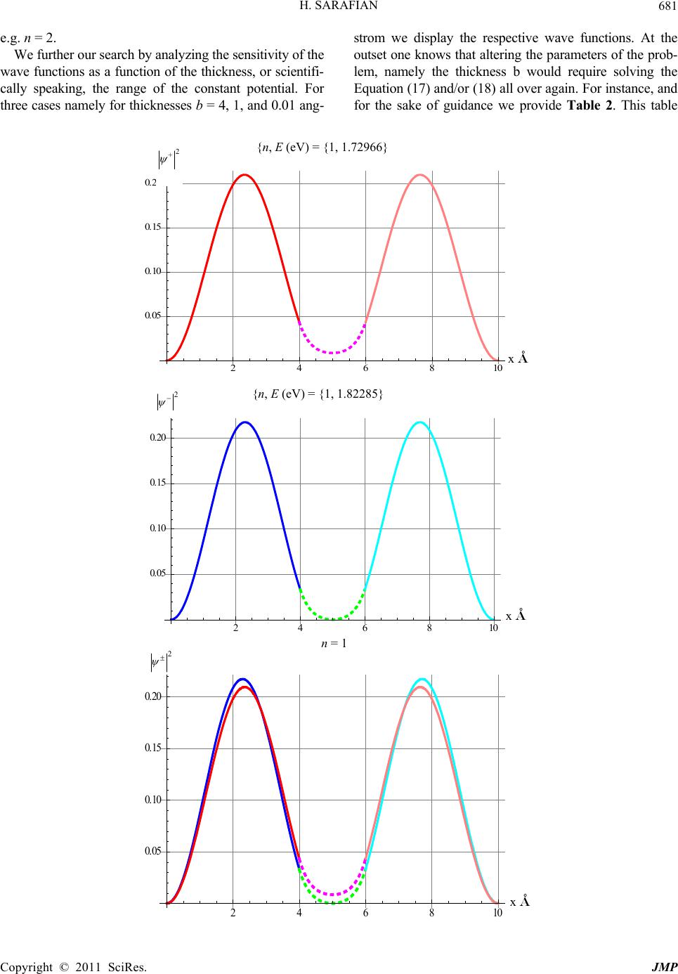

H. SARAFIAN681
e.g. n = 2.
We further our search by analyzing the sensitivity of the
wave functions as a function of the thickness, or scientifi-
cally speaking, the range of the constant potential. For
three cases namely for thicknesses b = 4, 1, and 0.01 ang-
strom we display the respective wave functions. At the
outset one knows that altering the parameters of the prob-
lem, namely the thickness b would require solving the
Equation (17) and/or (18) all over again. For instance, and
for the sake of guidance we provide Table 2. This table
2 4 6 810 x
A
°
0.05
0.10
0.1
5
0.20
2
n
,
E
eV 1, 1.72966
2 4 6 810 x
A
°
0.05
0.10
0.15
0.20
2
n
,
E
eV 1, 1.82285
2 4 6 810x
A
°
0.05
0.10
0.15
0.20
2
n
1
n, E ev
{n, E (eV) = {1, 1.72966}
{n, E (eV) = {1, 1.82285}
2
+

x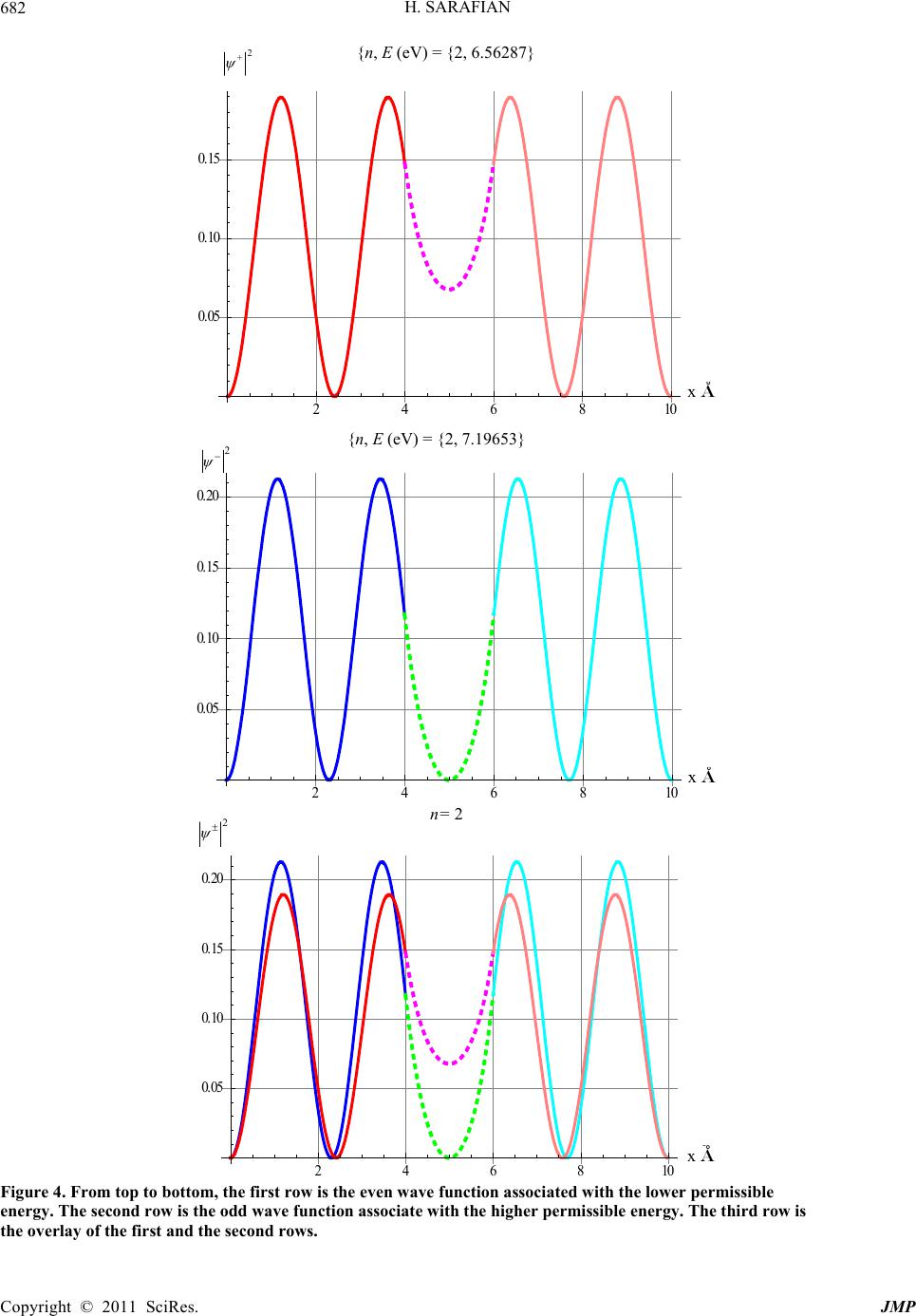
Å
2


x
Å
n = 1
2


x
Å

H. SARAFIAN 682
2 4 6 810x
A
°
0.05
0.10
0.1
5
2
n
,
E
eV
2
,6.56287
{n, E (eV) = {2, 6.56287}
2
+

246810 x
A
°
0.05
0.10
0.15
0.20
2
x
Å
n
,
E
eV
2
, .196537
{n, E7} (eV) = {2, .19653
2


2 4 6 810 x
A
°
0.05
0.10
0.15
0.20
x
Å
n
2
n= 2
2
2


x
Å
Figure 4. From top to bottom, the first row is the even wave function associated with the lower permissible
energy. The second row is the odd wave function associate with the higher permissible energy. The third row is
the overlay of the first and the second rows.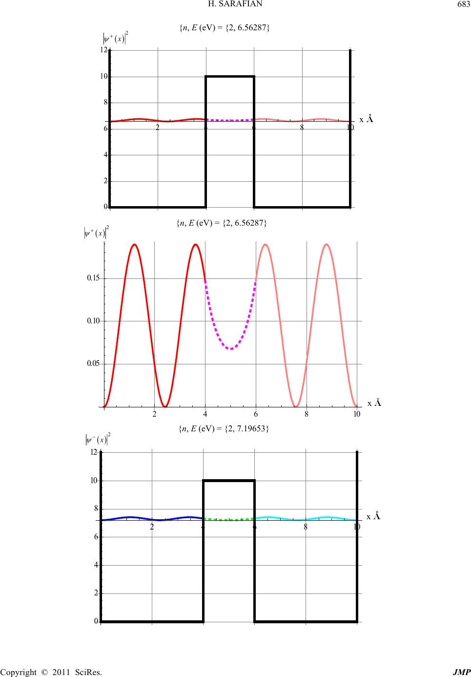

H. SARAFIAN683
2 4 6 810 x
A
°
0
2
4
6
8
1
0
1
2
x
n
,
E
eV
2
, 6.56287
{n, E (eV) = {2, 6.56287}
2
2 4 6 810 x
A
°
0.05
0.10
0.1
5
x
2
n,E eV
2
, 6.56287
2 46
8
10 x
A
°
0
2
4
6
8
10
12
x
2
n
,
E
eV
2
, 7.19653
x
Å
x
Å
x
Å
{n, E (eV) = {2, 6.56287}
{n, E (eV) = {2, 7.19653}

2


x

2


x

2


x

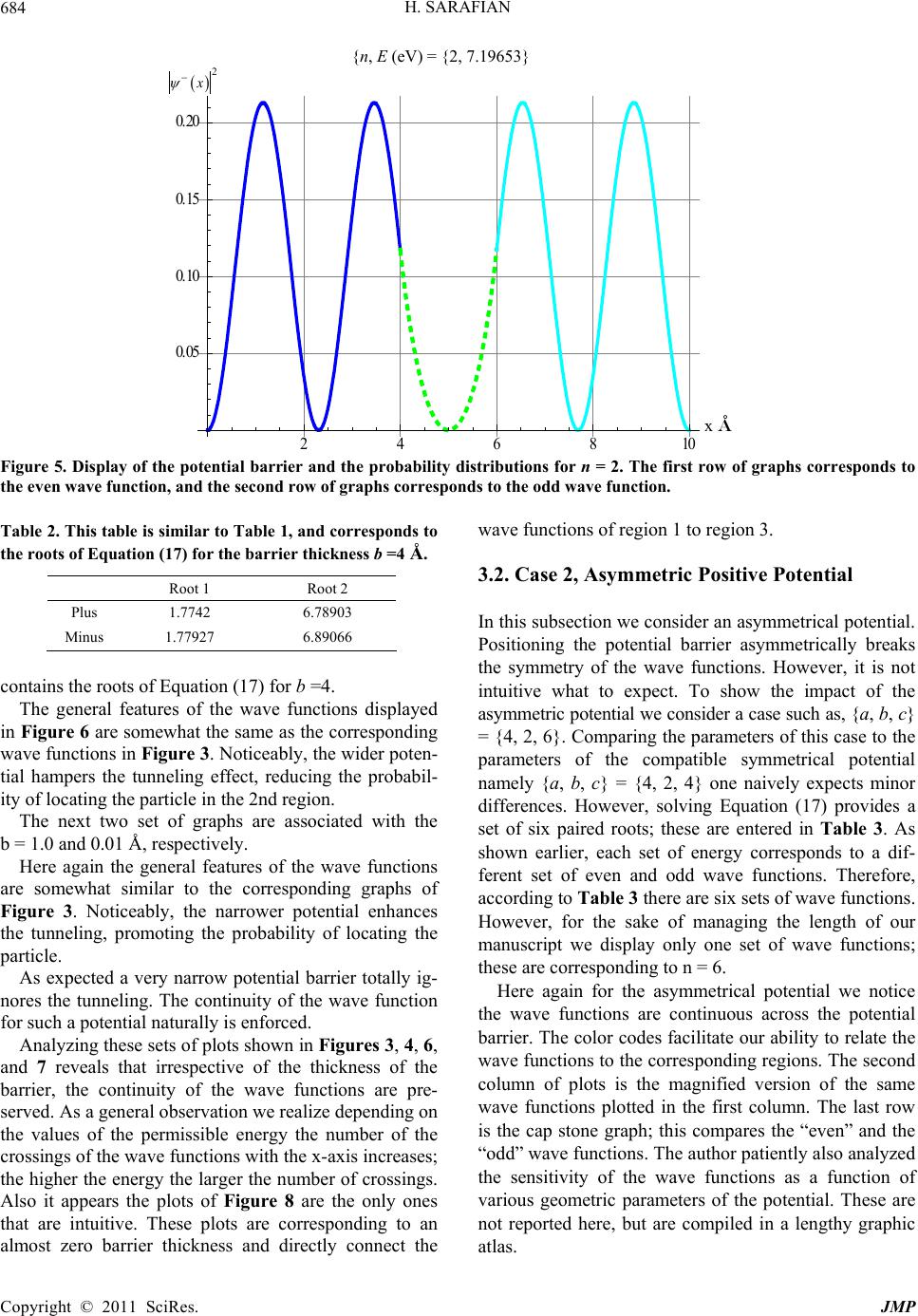H. SARAFIAN 684
246810 x
A
°
0.0
5
0.1
0
0.15
0.20
x
n
,
E
eV
2
, 7.19653
{n, E (eV) = {2, 7.19653}
2
Figure 5. Display of the potential barrier and the probability distributions for n = 2. The first row of graphs corresponds to
the even wave function, and the second row of graphs corresponds to the odd wave function.
Table 2. This table is similar to Table 1, and corresponds to
the roots of Equation (17) for the barrier thickness b =4 Å.
Root 1 Root 2
Plus 1.7742 6.78903
Minus 1.77927 6.89066
contains the roots of Equation (17) for b =4.
The general features of the wave functions displayed
in Figure 6 are somewhat the same as the corresponding
wave functions in Figure 3. Noticeably, the wider poten-
tial hampers the tunneling effect, reducing the probabil-
ity of locating the particle in the 2nd region.
The next two set of graphs are associated with the
b = 1.0 and 0.01 Å, respectively.
Here again the general features of the wave functions
are somewhat similar to the corresponding graphs of
Figure 3. Noticeably, the narrower potential enhances
the tunneling, promoting the probability of locating the
particle.
As expected a very narrow potential barrier totally ig-
nores the tunneling. The continuity of the wave function
for such a potential naturally is enforced.
Analyzing these sets of plots shown in Figures 3, 4, 6,
and 7 reveals that irrespective of the thickness of the
barrier, the continuity of the wave functions are pre-
served. As a general observation we realize depending on
the values of the permissible energy the number of the
crossings of the wave functions with the x-axis increases;
the higher the energy the larger the number of crossings.
Also it appears the plots of Figure 8 are the only ones
that are intuitive. These plots are corresponding to an
almost zero barrier thickness and directly connect the
wave functions of region 1 to region 3.
3.2. Case 2, Asymmetric Positive Potential
In this subsection we consider an asymmetrical potential.
Positioning the potential barrier asymmetrically breaks
the symmetry of the wave functions. However, it is not
intuitive what to expect. To show the impact of the
asymmetric potential we consider a case such as, {a, b, c}
= {4, 2, 6}. Comparing the parameters of this case to the
parameters of the compatible symmetrical potential
namely {a, b, c} = {4, 2, 4} one naively expects minor
differences. However, solving Equation (17) provides a
set of six paired roots; these are entered in Table 3. As
shown earlier, each set of energy corresponds to a dif-
ferent set of even and odd wave functions. Therefore,
according to Table 3 there are six sets of wave functions.
However, for the sake of managing the length of our
manuscript we display only one set of wave functions;
these are corresponding to n = 6.
Here again for the asymmetrical potential we notice
the wave functions are continuous across the potential
barrier. The color codes facilitate our ability to relate the
wave functions to the corresponding regions. The second
column of plots is the magnified version of the same
wave functions plotted in the first column. The last row
is the cap stone graph; this compares the “even” and the
“odd” wave functions. The author patiently also analyzed
the sensitivity of the wave functions as a function of
various geometric parameters of the potential. These are
not reported here, but are compiled in a lengthy graphic
atlas.
x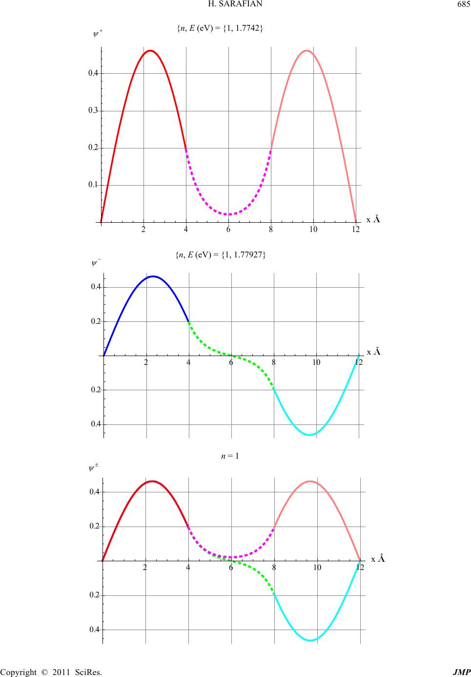
Å

2


x

H. SARAFIAN685
246810 12
n
,
E
eV 1, 1.7742
n, E ev
x A
°
0.1
0.2
0.3
0.4

 {n, E (eV) = {1, 1.7742}
2 4 681012 x
A
°
0.4
0.2
0.2
0.4
x
Å
n
,
E
eV 1, 1.77927
{n, E (eV) = {1, 1.77927}


x
Å
2 4 6 81
0
1
2
n
1
n = 1
x
A
°
0.4
0.2
0.2
0.4
x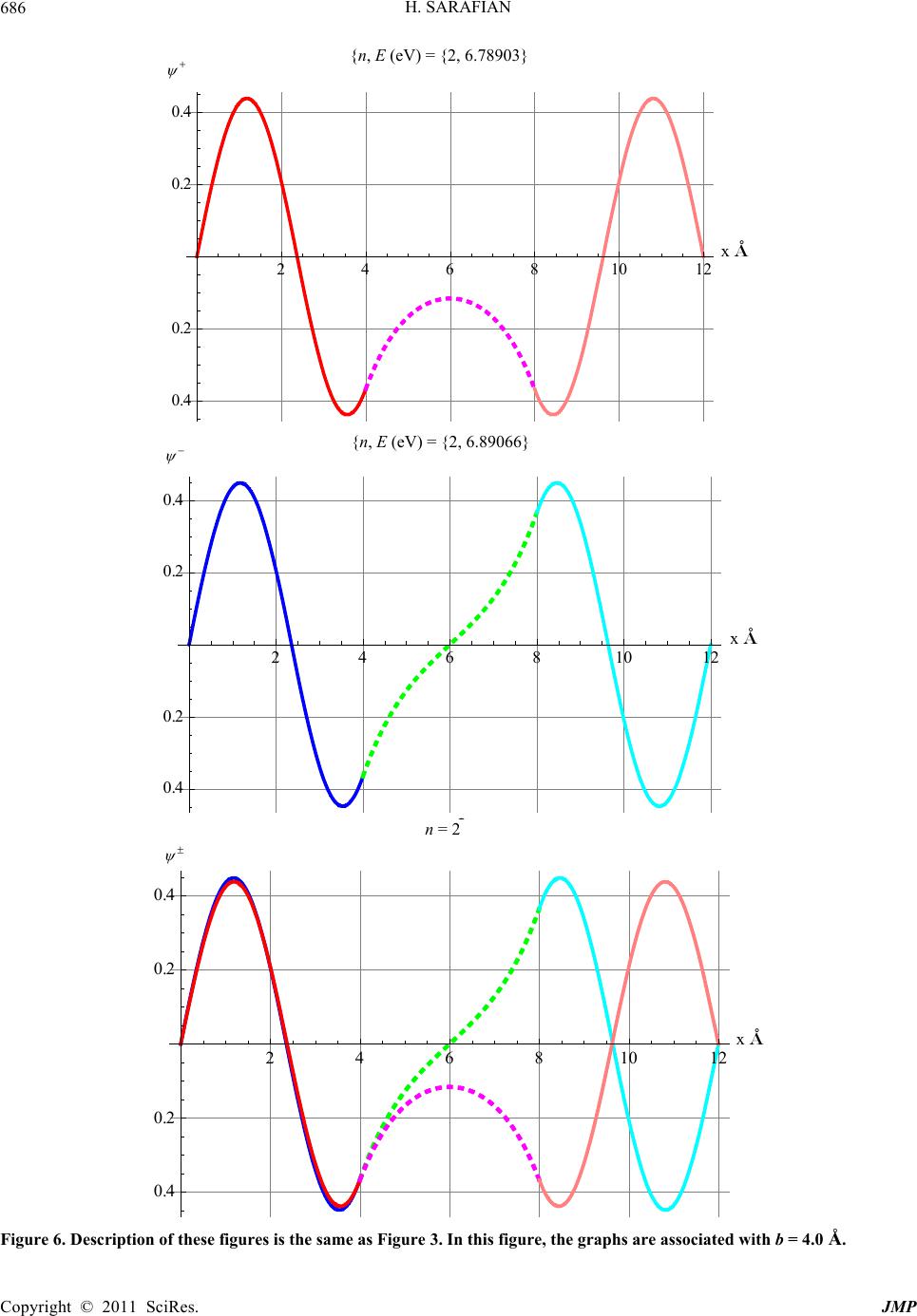
Å



H. SARAFIAN 686
2 4 6 81
0
1
2
n
,
E
eV
2
, 6.78903
n, E ev
x A
°
0.4
0.2
0.2
0.4
2 4 6 81012x
A
°
0.4
0.2
0.2
0.4
n
,
E
eV
2
, 6.89066
{n, E (eV) = {2, 6.78903}
{n, E (eV) = {2, 6.89066}


x
Å


x
Å
n
2
n = 2
2 4 6 81
0
1
2
x A
°
0.4
0.2
0.2
0.4
Figure 6. Description of these figures is the same as Figure 3. In this figure, the graphs are associated with b = 4.0 Å.
x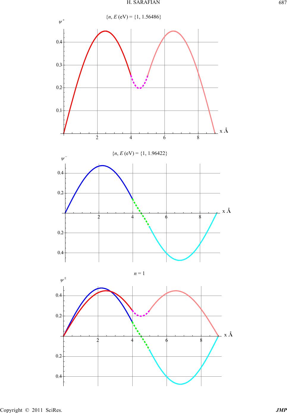
Å



H. SARAFIAN687
2
468x
A
°
0.1
0.2
0.3
0.4
n
,
E
eV 11.,56486
{n, E (eV) = {1, 1.56486}


x
Å
2 4 6 8
n
,
E
eV 1, 1.96422
{n, E (eV) = {1, 1.96422}
x A
°
0.4
0.2
0.2
0.4
2 4 6 8x
A
°
0.4
0.2
0.2
0.4
n 1 n = 1
x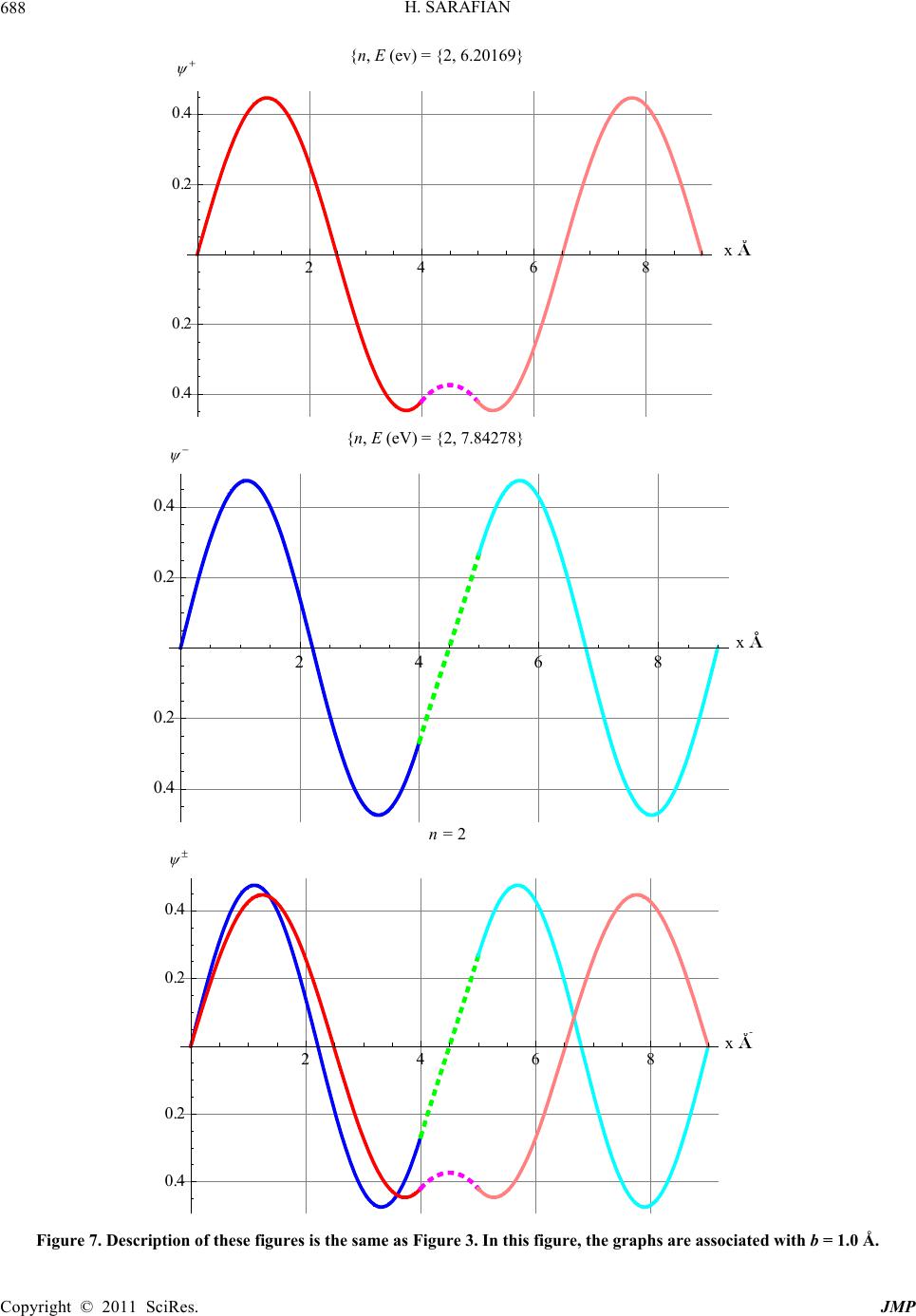
Å
x
Å





H. SARAFIAN 688
2 46 8
n
,
E
eV
2
, 6.20169
{n, E (ev) = {2, 6.20169}


x A
°
0.4
0.2
0.2
0.4
x
Å
n
,
E
eV
2
, 7.84278
{n, E (eV) = {2, 7.84278}
2468x
A
°
0.4
0.2
0.2
0.4
2 4 6 8x
A
°
0.4
0.2
0.2
0.4
n
2
Figure 7. Description of these figures is the same as Figure 3. In this figure, the graphs are associated with b = 1.0 Å.
x
Å
x
Å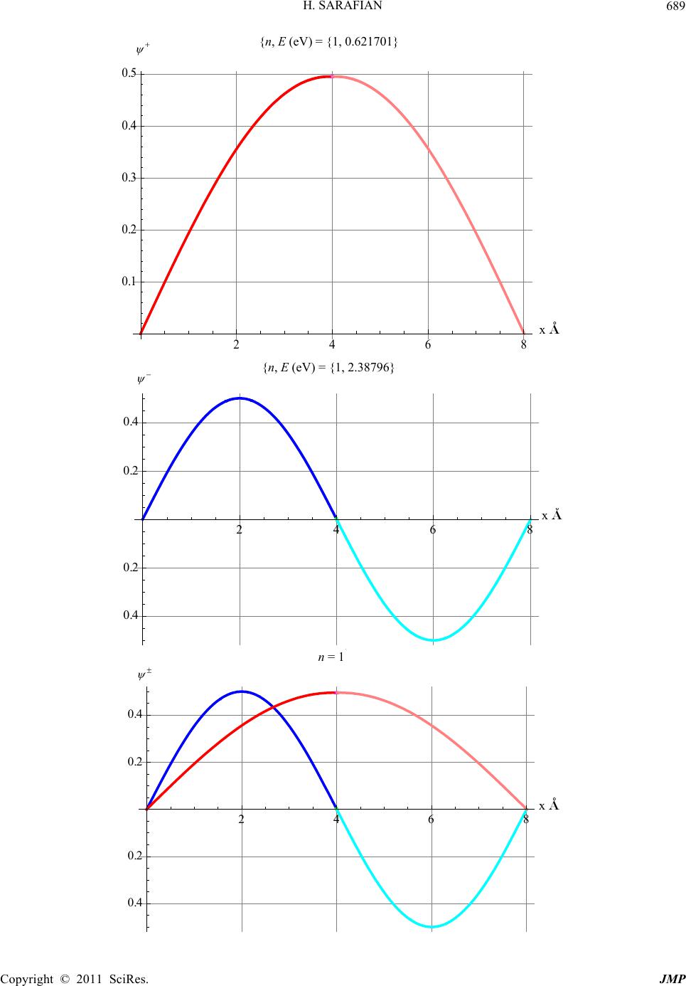
n = 2





H. SARAFIAN689
2 4 6 8
n,
E
eV 1, 0.621701
x A
°
0.1
0.2
0.3
0.4
0.5

 {n, E (eV) = {1, 0.621701}
2 46 8
x
Å
n
,
E
eV 1, 2.38796
{n, E (eV) = {1, 2.38796}


x A
°
0.4
0.2
0.2
0.4
x
Å
n
1
n = 1
2 46 8x
A
°
0.4
0.2
0.2
0.4
x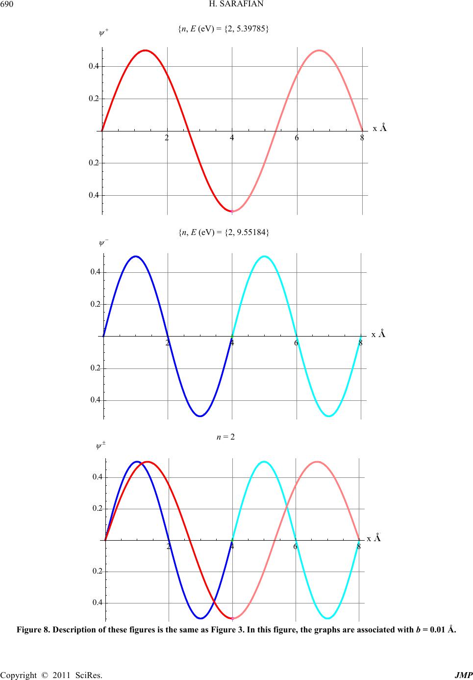
Å



H. SARAFIAN 690
2 46 8
n
,
E
eV
2
, 5.39785
{n, E (eV) = {2, 5.39785}


x A
°
0.4
0.2
0.2
0.4
x
Å
24 68
n
,
E
eV
2
, 9.55184
{n, E (eV) = {2, 9.55184}


x A
°
0.4
0.2
0.2
0.4
x
Å
24 68
n
2
n = 2


x A
°
0.4
0.2
0.2
0.4
x
Å
Figure 8. Description of these figures is the same as Figure 3. In this figure, the graphs are associated with b = 0.01 Å.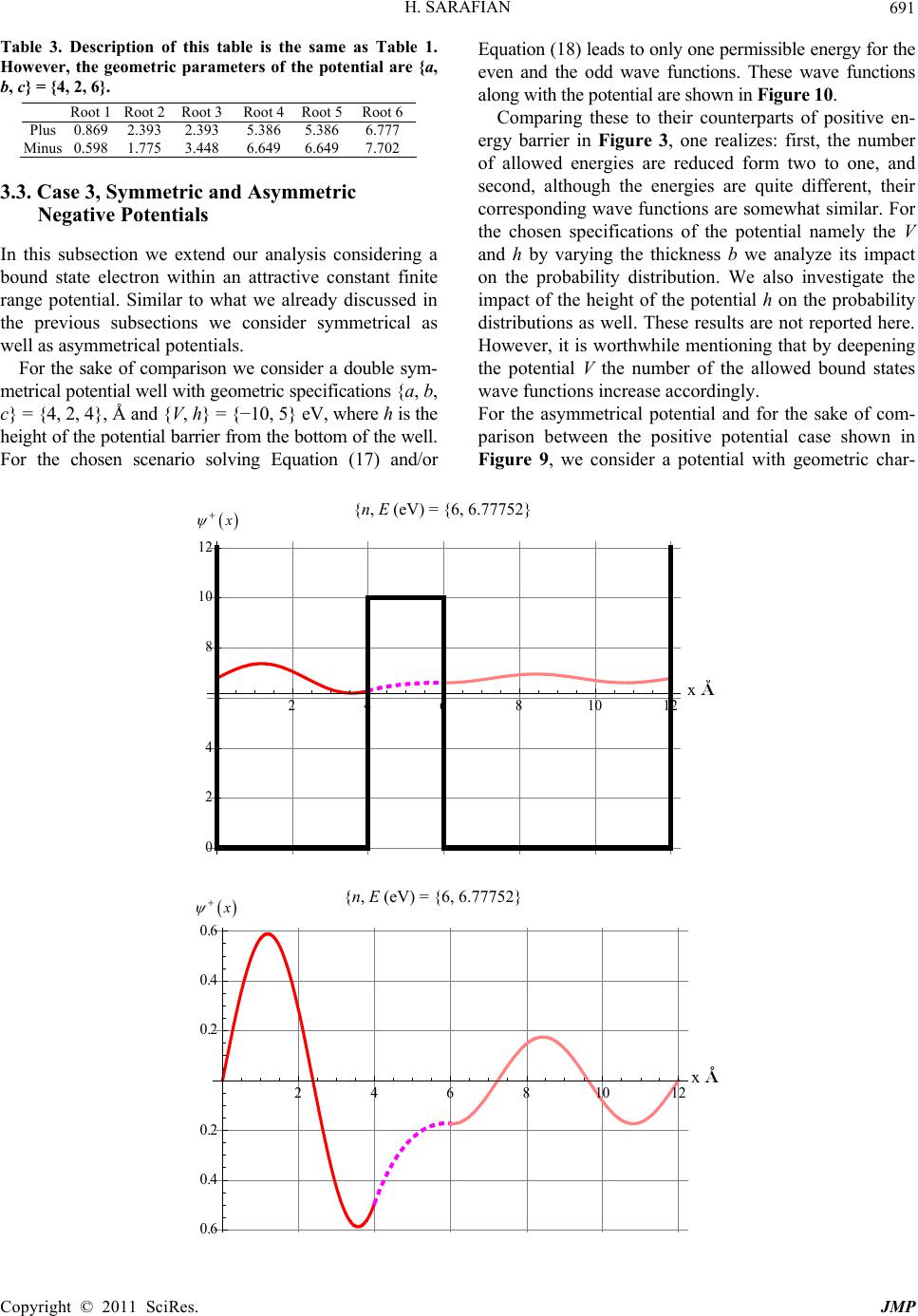

H. SARAFIAN691
Table 3. Description of this table is the same as Table 1.
However, the geometric parameters of the potential are {a,
b, c} = {4, 2, 6}.
Root 1 Root 2 Root 3 Root 4 Root 5 Root 6
Plus 0.869 2.393 2.393 5.386 5.386 6.777
Minus 0.598 1.775 3.448 6.649 6.649 7.702
3.3. Case 3, Symmetric and Asymmetric
Negative Potentials
In this subsection we extend our analysis considering a
bound state electron within an attractive constant finite
range potential. Similar to what we already discussed in
the previous subsections we consider symmetrical as
well as asymmetrical potentials.
For the sake of comparison we consider a double sym-
metrical potential well with geometric specifications {a, b,
c} = {4, 2, 4}, Å and {V, h} = {−10, 5} eV, where h is the
height of the potential barrier from the bottom of the well.
For the chosen scenario solving Equation (17) and/or
Equation (18) leads to only one permissible energy for the
even and the odd wave functions. These wave functions
along with the potential are shown in Figure 10.
Comparing these to their counterparts of positive en-
ergy barrier in Figure 3, one realizes: first, the number
of allowed energies are reduced form two to one, and
second, although the energies are quite different, their
corresponding wave functions are somewhat similar. For
the chosen specifications of the potential namely the V
and h by varying the thickness b we analyze its impact
on the probability distribution. We also investigate the
impact of the height of the potential h on the probability
distributions as well. These results are not reported here.
However, it is worthwhile mentioning that by deepening
the potential V the number of the allowed bound states
wave functions increase accordingly.
For the asymmetrical potential and for the sake of com-
parison between the positive potential case shown in
Figure 9, we consider a potential with geometric char-
2
4
68 1
0
12 x
A
°
0
2
4
8
1
0
12
x
n
,
E
eV
6
, 6.77752
{n, E (eV) = {6, 6.77752}



x
x
Å
2 4681
0
12
n,E eV 6, 6.77752
{n, E (eV) = {6, 6.77752}
x A
°
0.6
0.4
0.2
0.2
0.4
0.6
x



x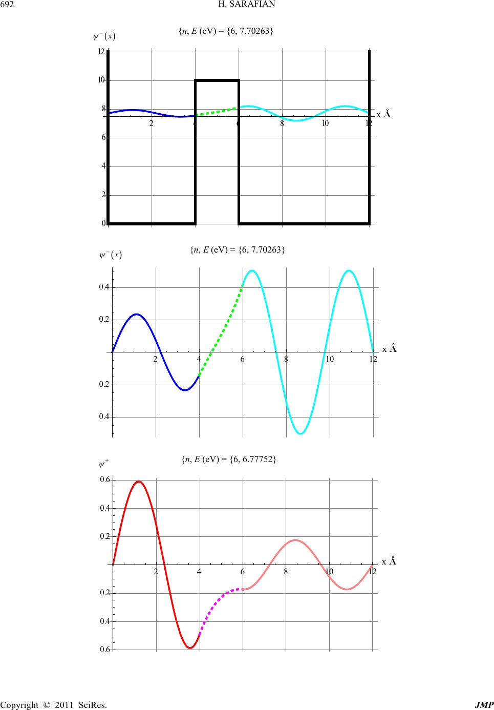
x
Å

H. SARAFIAN 692
2
4
68 1
0
12
x
A
°
0
2
4
6
8
1
0
12
x
n
,
E
eV
6
, 7.70263263
n, E ev
24681012 x
A
°
0.4
0.2
0.2
0.4
x
n
,
E
eV
6
, 7.70263
24681
0
12 x
A
°
0.6
0.4
0.2
0.2
0.4
0.6
n
,E eV 6, 6.77752
n, E ev
x
Å
x
Å
x
Å
{n, E (eV) = {6, 7.70263}
{n, E (eV) = {6, 7.70263}

x



x



 {n, E (eV) = {6, 6.77752}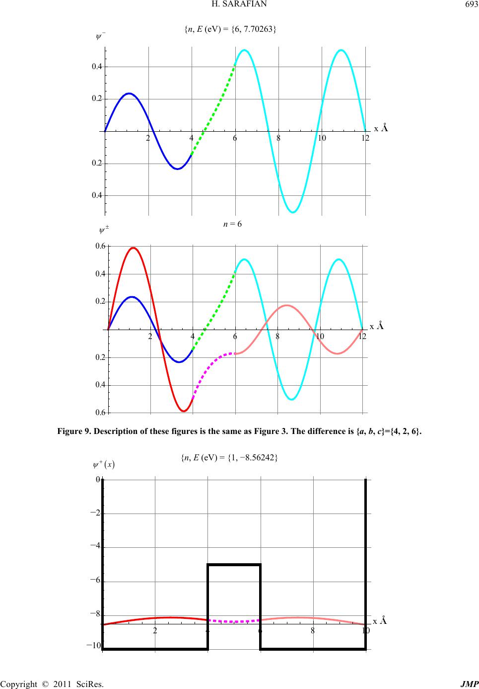

H. SARAFIAN693
2 4 6 810 12
n
,
E
eV
6
, 7.70263
{n, E (eV) = {6, 7.70263}


x A
°
0.4
0.2
0.2
0.4
x
Å
n
6
2 4 6 81
0
1
2
x A
°
0.6
0.4
0.2
0.2
0.4
0.6
Figure 9. Deption of these figus is the same as Figure 3. The difference is {a, b, c}={4, 2, 6}. scri re
24681
0
x A
°
1
0
8
6
4
2
0
x
n,E eV 1, 8.56242
n = 6


x
Å
{n, E (eV) = {1, −8.56242}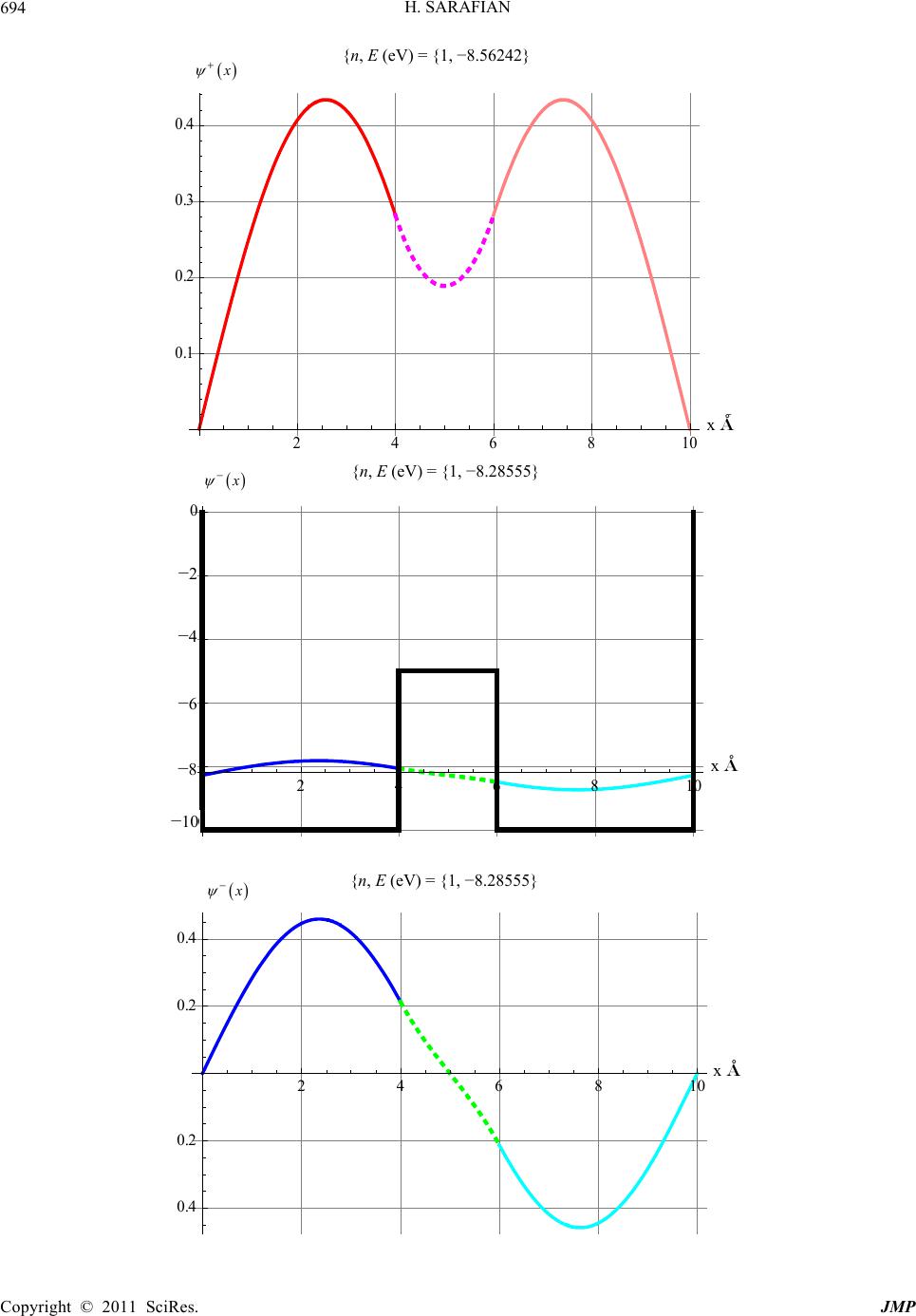

x


−2
−4
−6
−8x
Å
−10

H. SARAFIAN 694
2
468 10 x
A
°
0.1
0.2
0.3
0.4
x
n
,
E
eV 1, 8.56242
2 4 6 810 x
A
°
1
0
6
4
2
0
x
n
,
E
eV 1, 8.28555
2
4
68 10 x
A
°
0.4
0.2
0.2
0.4
x
n
,
E
eV 1, 8.28555
x
Å
x
Å
x
Å

x



x



x

 {n, E (eV) = {1, −8.28555}
{n, E (eV) = {1, −8.28555}
{n (eV) = {1 −8.56242}, E,
−2
−4
−6
−8
−10 −10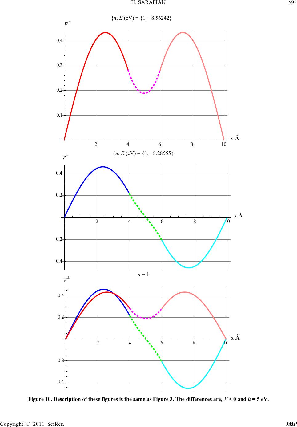

H. SARAFIAN 695
2
46810
n
,
E
eV 1,8.56242
{n, E (eV) = {1, −8.56242}


x A
°
0.1
0.2
0.3
0.4
x
Å
2
4
68 10
n
,
E
eV 1, 8.28555
{n () = {1 −8.28555}, EeV ,


x A
°
0.4
0.2
0.2
0.4
x
Å
n 1 n = 1


2
4
68 1
0
x A
°
0.4
0.2
0.2
0.4
x
Å
Figure 10. Description of these figures is the same as Figure 3. The differences are, V < 0 and h = 5 eV.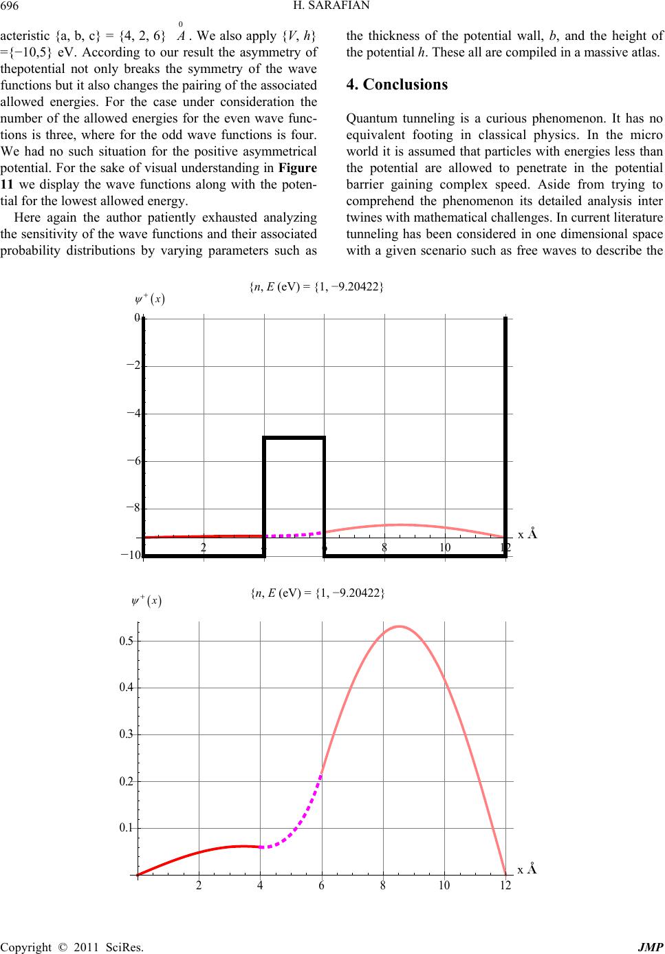

H. SARAFIAN 696
acteristic {a, b, c} = {4, 2, 6} 0
A
. We also apply {V, h}
={−10,5} eV. According to our result the asymmetry of
thepotential not only breaks the symmetry of the wave
functions but it also changes the pairing of the associated
allowed energies. For the case under consideration the
number of the allowed energies for the even wave func-
tions is three, where for the odd wave functions is four.
We had no such situation for the positive asymmetrical
potential. For the sake of visual understanding in Figure
11 we display the wave functions along with the poten-
tial for the lowest allowed energy.
Here again the author patiently exhausted analyzing
the sensitivity of the wave functions and their associated
probability distributions barying parameters such as
the thickness of the potential wall, b, and the height of
the potential h. These all are compiled in a massive atlas.
4. Conclusions
Quantum tunneling is a curious phenomenon. It has no
equivalent footing in classical physics. In the micro
world it is assumed that particles with energies less than
the potential are allowed to penetrate in the potential
barrier gaining complex speed. Aside from trying to
comprehend the phenomenon its detailed analysis inter
twines with mathematical challenges. In current literature
tunneling has been considered in one dimensional space
with a given scenario such as free waves to describe the y v
2
46810 12
x A
°
1
0
8
6
4
2
0
x
n
,
E
eV 1, 9.20422
2 4 6 81012 x
A
°
0.1
0.2
0.3
0.4
0.5
x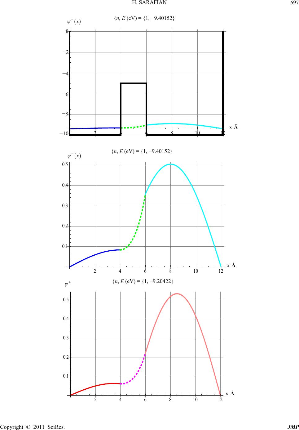
n
,
E
eV 1, 9.20422
{n, E (eV) = {1, −9.20422}
{n, E (eV) = {1, −9.20422}



x
−2
−4
−6
−8
x
Å
−10

x


x
Å

H. SARAFIAN697
2
468 1012x
A
°
1
0
8
6
4
2
0
x
n
,
E
eV 1,9.40152

x

 {n, E (eV) = {1, −9.40152}
−2
−4
−6
−8
24681012 x
A
°
0.1
0.2
0.3
0.4
0.5
x
x
Å
−10
n
,
E
eV 1, 9.40152
{n, E (eV) = {1, −9.40152}



x
x
Å
246810 12
n
,
E
eV 1, 9.20422
x A
°
0.1
0.2
0.3
0.4
0.5

 {n, E (eV) = {1, −9.20422}
x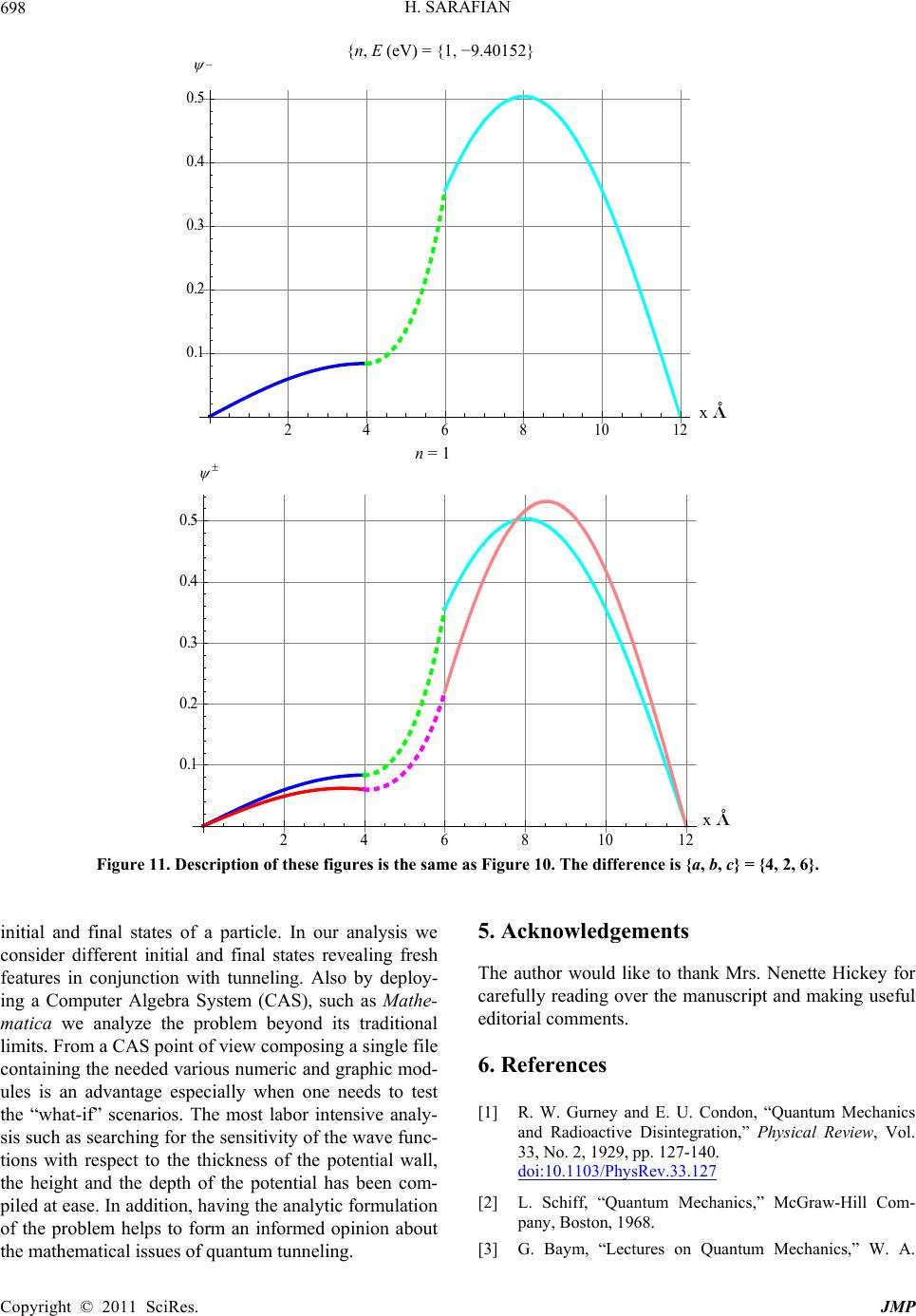
Å

H. SARAFIAN 698
2 4 6 81012
n,
E
eV 1,9.40152 {n, E (eV) = {1, −9.40152}
_

0.5
x A
°
0.1
0.2
0.3
0.4
x
Å
246810 12
n
1 n = 1


x A
°
0.1
0.2
0.3
0.4
0.5
x
Å
Figure 11. Description of these figures is the same as Figure 10. The difference is {a, b, c} = {4, 2, 6}.
5. Acknowledgements
initial and final states of a particle. In our analysis we
consider different initial and final states revealing fresh
features in conjunction with tunneling. Also by deploy-
ing a Computer Algebra System (CAS), such as Mathe-
matica we analyze the problem beyond its traditional
limits. From a CAS point of view composing a single file
containing the needed various numeric and graphic mod-
ules is an advantage especially when one needs to test
the “what-if” scenarios. The most labor intensive analy-
sis such as searching for the sensitivity of the wave func-
tions with respect to the thickness of the potential wall,
the height and the depth of the potential has been com-
piled at ease. In addition, having the analytic formulation
of the problem helps to form an informed opinion about
the mathematical issues of quantum tunneling.
The author would like to thank Mrs. Nenette Hickey for
carefully reading over the manuscript and making useful
editorial comments.
6. References
[1] R. W. Gurney and E. U. Condon, “Quantum Mechanics
and Radioactive Disintegration,” Physical Review, Vol.
33, No. 2, 1929, pp. 127-140.
doi:10.1103/PhysRev.33.127
[2] L. Schiff, “Quantum Mechanics,” McGraw-Hill Com-
pany, Boston, 1968.
[3] G. Baym, “Lectures on Quantum Mechanics,” W. A.

H. SARAFIAN699
Benjamin, Inc., New York, 1976.
[4] A. S. Davydov, “Quantum Mechanics,” 2nd Edition,
Pergamon Pr., Mesland, 1976.
[5] E. Merzbacher, “Quantum Mechanics,” 3rd Edition,
Wiley, Hoboken, 1997.
[6] http://www.youtube/QM5.1,QM5.4,QM6.1 and QM6.3
[7] J. M. Feagin, “Quantum Methods with Mathematica,”
Springer-Verlag, Berlin, 1994.
[8] Wolfram demonstration Projects, April 2011.
http://demonstrations.wolfram.com.
[9] S. Wolfram, “The Mathematica Book,” 4th Edition,
Cambridge University Press, Cambridge, 1999 and
“MathematicaTM” software V8.0, 2010.
[10] N. J. Giordano and H. Nakanishi, “Computational Phys-
ics,” 2nd Edition, Pearson, Prentice Hall, Upper Saddle
River, 2006.