Applied Mathematics, 2011, 2, 816-823
doi:10.4236/am.2011.27109 Published Online July 2011 (http://www.SciRP.org/journal/am)
Improved Ostrowski-Like Methods Based on Cubic
Curve Interpolation
Janak Raj Sharma1, Rangan Kumar Guha1, Rajni Sharma2
1Department of Mat hem at i cs, Sant Longowal Institute of Engineering and Technology, Longowal, India
2Department of Appli e d Sci en ces , D.A.V. Institute of Engineering and Techno logy Kabirnagar, Jalandhar, India
Received December15, 2010; revised May 10, 2011; accepted May 13, 2011
Abstract
In this paper, we derive two higher order multipoint methods for solving nonlinear equations. The method-
ology is based on Ostrowski’s method and further developed by using cubic interpolation process. The adap-
tation of this strategy increases the order of Ostrowski’s method from four to eight and its efficiency index
from 1.587 to 1.682. The methods are compared with closest competitors in a series of numerical examples.
Moreover, theoretical order of convergence is verified on the examples.
Keywords: Nonlinear Equations, Ostrowski’s Method, Root-Finding, Order of Convergence, Cubic
Interpolation
1. Introduction
Finding the root of a non-linear equation () 0fx

is a
common and important problem in science and engi-
neering. Analytic methods for solving such equations are
almost non-existent and therefore, it is only possible to
obtain approximate solutions by relying on numerical
methods based on iteration procedures. Traub [1] has
classified numerical methods into two categories viz. 1)
one-point iteration methods with and without memory,
and 2) multipoint iteration methods with and without
memory. Two important aspects related to these classes
of methods are order of convergence and computational
efficiency. Order of convergence shows the speed with
which a given sequence of iterates converges to the root
while the computational efficiency concerns with the
economy of the entire process. Investigation of one –
point iteration methods with and without memory, has
demonstrated theoretical restrictions on the order and
efficiency of these two classes of methods (see [1]).
However, Kung and Traub [2] have conjectured that
multipoint iteration methods without memory based on
evaluations have optimal order . In particular,
with three evaluations a method of fourth order can be
constructed. The well-known Ostrowski’s method [3] is
an example of fourth order multipoint methods without
memory which is defined as
n1 2n


,
i
ii i
f
x
wx
f
x




   
1,
2
ii
ii ii i
fw fx
xw
f
xfx fw

 (1)
where 0,1,2,i

 and 0
x
is the initial approximation
sufficiently close to the required root. The method re-
quires two function
f
and one derivative
f

evalua-
tions per step and is seen to be efficient than classical
Newton’s method.
Recently, based on Ostrowski’s method (1) Grau and
Díaz-Barrero [4] have developed a sixth order method
requiring four evaluations, namely three
f
and one
f

per iteration. Sharma and Guha [5] have shown that
there exists a family of such sixth order methods with
equal number of evaluations.
In the present paper, we derive two modified Os-
trowski’s-type methods which improve the local order of
convergence from four for Ostrowski’s method to eight
for new methods. The important feature of these methods
is that per step they require three evaluations of
f
and
one evaluation of
f

. Thus, the new methods support
the conjecture of Kung and Traub for eighth order
methods based on four evaluations.
The paper is organized in six sections. In Section 2,
methods are developed and their eighth order conver-
gence is established. In Section 3, computational effi-

J. R. SHARMA ET AL. 817
ciency of the methods is discussed. Section 4 contains
the numerical experimentations and comparison with
some well known methods. Concluding remarks are given
in Section 5. In Section 6, references are given.
2. The Methods and Their Convergence
Method One
Consider the Ost rowski schem e (1) now defined by





 
,
.
2
i
ii i
ii
ii ii i
fx
wxfx
fw fx
zw
f
xfxfw




(2)
In what follows, we construct the method to obtain the
approxim ation 1i
x
 to the root by considering the cubic
curve interpolation. Let


23
,
ii
yx abxxcxxdxx 
i
(3)
be an interpolatory p ol y nom i a l of degree t h ree such that



,
ii
y
xfx (4)



,
ii
y
xfx

 (5)



,
ii
y
wfw (6)



,
ii
y
zfz (7)
and



.
ii
y
zfz

 (8)
Our interest is to find the unknown parameters a, b, c
and d introduced in the polynomial. In order to achieve
that, we make use of the expressions (4) - (7) in (3). From
(3), (4) and (5), it is easy to show that

(),
.
i
i
afx
bfx


 (9)
Substituting the values of a and b in (3) then using (6)
and (7), we obt ain after some simple calculati ons
() () 1
() ()
ii
ii i
ii ii
fw fx
cdw xfx
wx wx


 


, 
(10)
  
1.
ii
ii i
ii ii
fz fx
cdzxfx
zx zx


 



(11)
Solving these equations using Ostrowski iteration (2),
we obtain

   
 
2
2
2,
iii
i
iii i
fxfx fw
cfw
fx fw fxfw


 








  
3
32
2,
iii
iii i
fxfx fw
dH
fxfw fxfw

 (13)
where
 

   
     
3
2
2.
iiiiii
iii i
Hfxfwfxfw fxfw
fx fzfxfw

 

.
The tangent line to the curv e of cubic polyn omial (3) at
the point




,
ii
zyz is given by


.
ii

i
y
yzy zxz

  (14)
Assuming that the root estimate 1i
x
 is point of inter-
section of the tangent line (14) with x-axis, then


10. i
yx


Thus , fr om (7), (8) and (14 ), we o btain


1.
i
ii i
fz
xz
yz

 (15)
Now using the approximation (8) in (15), we can ob-
tain the new improvement as given by


1.
i
ii i
fz
xz
fz

 (16)
where i is the Ostrowski point. It is quite obvious that
formula (16) together with (2) requires five evaluations
per iteration. However, we can reduce the number of
evaluations to four by utilizing the approximation (8).
Therefore, (3) and (8) yield
z
  
2
23
iiii ii
fzyzbczxdzx

. (17)
Substituting the values of c and in (17), we
obtain ,bd




,
ii

i
f
zyzfx 

 (18)
where
    
       


 



 

3
2
1
22
2
2.
ii iiii
ii iii
ii i
ii iiii
fwfwfxfx fzfw
fxfxfwf wfz
fx fxfw
fx fwfwfxfxfw
 














Then the formula (16) in its final form is given by



1
1,
i
ii i
f
z
xz
f
x


  (19)
where is the Ostrowski iteration (2) and
i
z

is given
in (18).
2
H




(12)
Thus, we derive a multipoint method based on the
composition of two sub steps, Ostrowski sub step (2) fol-
lowed by (19) obtained by tangential cubic interpolation.
It is straight forward to see that per step the method util-

J. R. SHARMA ET AL. 818
izes four pieces of information namely-

,
i
f
x


,
i
f
x


i
f
w and

.
i
f
z Since we are using the approxima-
tion (8) for the derivative, therefore the error is given by
(see [6])
Theorem 1. Let


f
x be a real valued function. As-
suming that


f
x is sufficiently smooth in an interval I.
If


f
x has a simple root
I

 and 0
x
is suffi-
ciently close to

then the method defined by (19) is of
order eight.
 



2,
4!
iv
ii iii
f
fz yzzx zw


 

i

(20)
where .
iii iii

min,, ,max,,
x
wz xwz 
 
In order to
show that the method is of order eight, we prove the fol-
lowing theorem:
Proof: Let ,
ii
ex


 ii ew


 and ˆii
ez



be errors in the ith iteration. Using Taylor’s series expan-
sion of


i
f
x about

and taking into account that


f  0

and


0,f 


we have




23456 7
23456,
iiiiiii
fxfeAeAeAeAeAeO e 




i
(21)
where





1!,2,3,
k
k
Akff k 


Furthermore, we have
 


23456
234 56
123456
iiiiii
fxfAeAeAeAeAe Oe 

 

.
i
(22)



 

223 3422
23243225423322
22 3567
65243 423232 2
23744106208
513 1728335216.
iii ii
i
ii
fx eAeAAeA AAAeAAA AAA Ae
fx
AAAAAAA AAAAAeOe
 

 


45
i
(23)
Substitution of (23) in first step of (2), yields




223 3422
232 43225423322
22 3567
65243 423232 2
23744106208
513 172833 5216.
ii ii
ii
eAeAAeAAAAeAAAAAAAe
AAAAAAA AAAAAeOe
  
   


45
i
(24)
Expanding

i
f
w about

an d using ( 24) , we obtain
 

 



223 3422
232 43225423322
22 3567
652434232 322
23754 1062412
513 1734377328.
ii ii
ii
45
i
f
wfAeAAeAAAAeA AAAAAAe
AAAAAAAAAAAAeOe


 


 
(25)
Using Equations (21), ( 23) an d ( 25) , we obta i n



 
 

2233422
232 43225423322
22 3567
6524342 32 322
22 363 484124
2
510 10 1615226.
ii ii i
ii i
ii
fx fw


45
i
A
eAAeAAAAeAAAAAAA
fxfx fw
AAAAAAAAAAAAeOe
 

  
e
(26)
From second step of (2) it follows that




34 2245
232423322
22 3567
524342 32 32 2
ˆ2284
3 7121830 10.
ii i
ii
eAAAeAAAAAAe

A
AAA AAAAAAAeOe

 
(27)
Expanding

i
f
z about ,

we obtain






29
2
ˆˆ ,
iii
fzfeAeOe 
i





 (28)
Using (27) in (28) , we get

J. R. SHARMA ET AL. 819
 




34 2245
232423322
22 3567
52434232322
2284
3 7121830 10.
ii i
ii
f zfAAA eAAAAAAe
AAAAAAAAAAAeO e






 

2,
(29)
Using the results of (21), (25) and ( 29) in
 

 

 

 

 

 

 

3
1
2
2
22
ii iiii i ii
iiii iiiiii i
fwfwfxfx fzfwfxfxfw
fw fzfxfxfwfxfw fwfxfxfw
 


 


 
 
 
and simplifying, we get



22332 244
223 43225423322
124 341285179 3818.
ii ii

5
i
A
eAAe AAAAeAAAAAA AeOe    (30)
From (22) and (30 ), we get
 




345
24 32 2
122
i
fxfAAAAAe Oe  .
ii





 (31)
Using (28) and (3 1) in



1
1,
i
ii i
f
z
xz
f
x


  we find the er ror eq uation as give n by

 

 
29
223
1224322
345
24 322
2349
224322
2
33389
22 3224322 2 32
2
2
ˆˆ
ˆˆˆˆ 122
122
ˆˆ
22
22
ii i
iiiiiii
ii
iiii
ii
eAeOe
eeeeAe AAAAAeOe
AAAAAe Oe
AeAAAAAeeOe
AAAAAAAAA A AAeOe
AA



 

 



 


 


 



 
22 89
23223 4. ii
AAAA AeOe




49
(32)
Thus Equation (32) establishes the maximum order of
convergence equal to eight for the iteration scheme de-
fined by (19). This completes the proof of the theorem.
Remark 1. The error (20) is now given by
 



2
ˆˆ .
4!
iv
iiii ii
f
f
zyz eeee


  
From (24), (27) and Taylor’s expansion of


iv
f

about ,

we can obtain the error as
 

45
42 . ii ii
f
zyz AAeOe

  (33)
This shows that the error in derivative approximation
is of order four.
Remark 2. Upon using Taylor’s expansion

i
fz



2
2ˆˆ
12 ii
f
AeO e 


 
i



,

in (33), we get



45
242
ˆ
12 ,
iii
yzfAe AAeOe 




that is



34 5
24 32 2
122
i
ii
yz
fAAAAAeOe 





(34)
which is same as obtained in equation (31) of




.
ii
y
zfx 

 This verifies the correctness of error
(33) and calculation of


i
y
z
.
Remark 3. From the convergence theorem of iterative
functions [1], if


1
g
x and

2
g
x
p

are two iterative
functions of order 1 and 2, respectively, then the
new composite iterative function
p

 
21
gg x

Gx
i
z
has
the order 12 In our case, the Ostrowski method (2)
comprising the first two steps, is of order four. Thus to
produce eighth order method the formula (19) should be
of order two (neglecting how is obtained). From (34),
it turns out that
.pp

 


1.e

ˆˆ
Ae
ˆ
f O 


3
ii
f x



2
ˆ
.Oe
i

Also, the Taylor’s series expansion of the func-
tion 2
iiii
yz

e

ffz 






 On substitution
and simplifying, we see that the Newton-like method (15)
and hence (19), has the order two, thus verifying the con-
vergence theorem on composition of two iterative func-
tions to produce eighth order i t erative me thod.
2.2. Method Two
Here we consider the inverse interpolation. Let

J. R. SHARMA ET AL. 820

   







2
3,
i
i
i
F
fxABfx fx
Cfx fx
Dfx fx
 


(35)
be an inverse interpolatory polynomial of degree three
such that



,
ii
F
fx x (36)



1,
ii
Ffx fx

 (37)



,
ii
F
fw w (38)



,
ii
F
fz z

(39)
and



1.
ii
Ffz fz

 (40)
From (36) and (37), we can calculate
A
and as
given by B

,1
i. i
A
xB fx

 (41)
Substituting the values of
A
and in (35), then
using (38) and (39 ), we o btain B
 


 



2
1
ii
i
i
ii
CDfw fx
fw
fx
fw fx

 

(42)
and
 

  



 


2
1
.
2
ii
ii
ii i
iiii
C Dfzfxfz fx
fw fxfz
fxfxfwfx









(43)
The Equations (42) and (43) when solved, yield
  



 
 
2
1
1,
i
i
ii
ii
ii i
f
w
C
f
x
fw fx
fw fxG
fxfwfz
 



(44)
 
1,
ii i
DG
fx fwfz
 (45)
where


  
 

  
 
2
2
1.
2
i
ii
ii
iii
ii
fw
Gfw fx
fx fw
fz fx fw
fz fx
 






The tangent line to the curve of cubic polynomial (35)
at the point






,
ii
F
fzfz is given by
















.
ii i
F
fxFfzF fzfxfz

 
The approximation to the ro ot 1i
x
 is now obtained by
intersecting this tangent line with x-axis. This yields


1,
i
ii i
f
z
xz
f
z

 (46)
where




 

  
1
2
1
2
3.
ii
ii
ii
fz Ffz
BCfzfx
Dfz fx



 





From (40), (44 ) and (45), we have
 
11
,
ii
f
zfx
 

(47)
where

 
 
 
 
  
 
2
1
12
.
2
ii
iii i
ii ii
ii
iii
fwfz fx
fw fzfw fz
fw fzfz fx
fx fw
fz fw fw



 



i
















Hence, the iteration formula (46) is gi ven by


1,
i
ii i
f
z
xz
f
x

  (48)
where is the Ostrowski iteration (2) and
i
z

is shown
in (47).
Thus, we obtain second modified Ostrowski-like me-
thod (48) devel oped by t a ngen t i al i nverse i nte rpol at i on. I n
this method also, the number of evaluations required is
same as in the first method. Error in the approximation
(40), likewise the error ( 20 ), can be given by
 


    
() 2
1
,
4!
i
i
iv
iii i
Ffz
fz
ffz fxfz fw 




(49)
where
 


  

min, ,,
max, ,.
iii
iii
f
xfwfz
fxfwfz






J. R. SHARMA ET AL. 821
In the following theorem we prove that the method is
of order eight.
Theorem 2. Under the hypotheses of theorem 1, the it-
eration method defi ned by (4 8) is of order eig ht .
Proof: Using (21), (25) and (29), after simple calcula-
tions we find
 




 



223244 5
232 432542232
12
2
146 28 410 622.
ii
i
ii iiii
ii ii
fw fx
fz
fw fzfzfxfxfw

i
A
eAAeAAAe AAAAAAeOe



 


  
(50)
Also

 
 
 



2
2232 445
23 24 32642232
1232445.
iii
ii i i
ii ii
fwfzfx
fwfz fwfx

i
A
eAAeAAAe AAAAAAeOe






 
(51)
From (47) we know 1Equation (50)Equation (51)

 , which implies


23 244
23 4542322
12 34577.
ii iii

5
A
eAe AeAAAAA AeOe    (52)
From (22) and (52 ), we get
 




34 5
24 32 2
1177
ii
i
AA AAAeOe
fx f.







 (53)
Then using (28 ) and (5 3) in


1,
i
ii i
f
z
xz
f
x

  we obtain the error equation








292 445
12 42232
22449
242232
2349
2 24322
2
333
22 32243222 32
ˆˆ ˆ177
ˆˆ ˆ
177
ˆˆ
77
77
iiii iii
ii iii
iiii
ii
eeeAeOe AAAAAeOe
eeAeAAAA Ae Oe
AeAAAAAeeOe
8
A
AAAAA AA AAAAeOe

 



 



 


 






 
9
2228 9
22 322 34
6.
ii
AA AAA AAeOe

 

(54)
This result shows the eighth order convergence of
method (48).
Remark 4. The error (49) upon using (21), (25) and
(29) is given by
 


 


345
2
1
.
4!
i
i
iv
ii
Ffz
fz
FfAeOe 





 


Expanding


iv
F

about

and using the fact that
 


 






 
3
()
765
3
2324
4
15 10
(0)
4!
55,
iv
iv fff f
Ffff
AAAA
f






 
 





we can obtain the error as
 



34 5
24 32 2
1
155
i
i
ii
Ffz
fz
.
A
AAAAeOe
f 







(55
in approximation (40) is of
orRemark 5. Upon using Taylor’s expansion
)
This shows that the error
der four.


1i
f
z




2
2ˆˆ
112
ii
f
AeO e 






in (55), we get






345
1ˆ
125 5,Ae AAAAAeO e

224322
i
ii i
Ffz

f





that is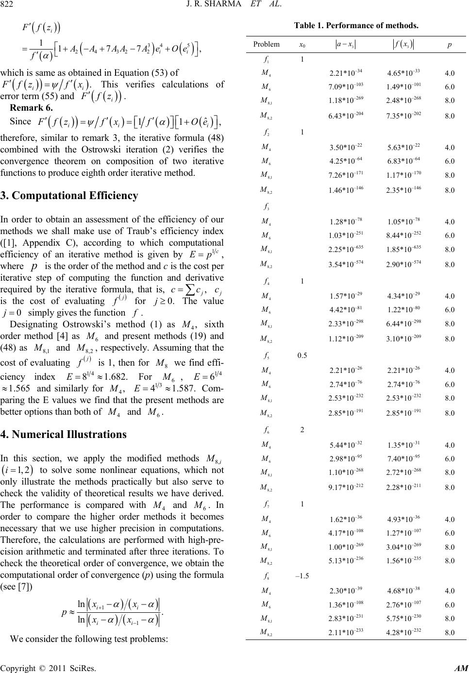


J. R. SHARMA ET AL. 822





34 5
24 32 2
1177
i
ii
Ffz
AA AA AeOe
f 





,


which is same as obtained in Equation (5 3) of




.
ii
F
fzf x 

 This verifies calculations of
rm (55) and error te


i
F
fz
.
Remark 6.
Since


 


ˆ
11
ii ,Ffzfx fO



 


therefore, similar to remark 3, the iterative formula (48)
combined with the Ostrowski iteration (2) verifies the
iterative
functions to prod uce ei g
3. Computational Efficiency
i
e
convergence theorem on composition of two
hth order iterat i ve met hod.
In order to obtain an assessment of the efficiency of our
methods we shall make use of Traub’s efficiency index
([1], Appendix C), according to which computational
efficiency of an iterative method is given by 1c Ep,
where
p
is the order of the method and c is the cost per
ction and derivative
at is,
iterative step of computing the fun
required by the iterative formula, th,
j
cc

j
c
is the cost of evaluating

j
f
for 0.j The value
0j simply gives the funct ion
f
.
Designating Ostrowski’s method (1) as 4,
M
sixth
order method [4] as 6
M
and present methods (19) and
(48) as 8,1
M
and 8,2
M
, respectively. Assuming that the
cost of evaluating

j
f
is 1, then for 8
M
we find effi-
ciency index 14 8 1.682.E For 6
M
, 14 6
1.565 and similarly for E
4,
M
13 4
esent m
1
hrethods are
.587.E Com-
the E values we find that te pparing
better options t han bot h of 4
M
and 6
M
.
4. Numerical Illustrations
In this section, weply the modified methods ap8,i
M

1, 2i to solve some nonlar equaich not
only illustrate the methods practically but also serve to
check the validity of theoretical results we have derived.
The performance is comp4
inetions, wh
ared with
M
and 6
M
. In
mes order to compare the higher ord
necessary that we use higher preer ms it cision in computations.
pre-
ethod beco
Therefore, the calculations are performed with high-
cision arithmetic and terminated after three iterations. To
check the theoretical order of convergence, we obtain the
computational order of convergence (p) using the formula
(see [7])

 
1
1
ln .
ln
ii
ii
xx
pxx








Table 1. Performance of methods .
Problem x0 3
ax

3
f
x p
1
f
1
4
M
2.21*10–34 4.65*10–33 4.0
6
M
7.09*10–103 1.49*101 6.0 0–1
8,1
M
1.18*10–269 2.48*10–268 8.0
8,2
M
6.43*10–204 7.35*10–202 8.0
2
f
1
4
M
3.50*10 5.63*10–2
–2224.0
6
M
4.25*10–64 6.83*10–64 6.0
8,1
M
7.26*10–171 1.17*10–170 8.0
8,2
M
1.46*10–146 2.35*10–146 8.0
3
f
4
M
1.28*108 1.
–7 8
05*10–7 4.0
6
M
1.03*0–251 8.44*0–252 6.
110
8,1
M
2.25*10–635 1.85*10–635 8.0
8,2
M
3.54*10–574 2.90*10–574 8.0
4
f
1
4
M
1.57*109 4.
–2 9
34*10–2 4.0
6
M
4.42*10–81 1.22*10–80 6.0
8,1
M
2.33*10–298 6.44*10–298 8.0
8,2
M
1.12*10–209 3.10*10–209 8.0
5
f
0.5
4
M
2.21*106 2.
–2 6
21*10–2 4.0
6
M
2.74*10–76 2.74*10–76 6.0
8,1
M
2.53*10–232 2.53*10–232 8.0
8,2
M
2.85*10–191 2.85*10–191 8.0
6
f
2
4
M
5.44*102 1.
–3 1
35*10–3 4.0
6
M
2.98*10–95 7.40*10–95 6.0
8,1
M
1.10*10–268 2.72*10–268 8.0
8,2
M
9.17*10–212 2.28*10–211 8.0
7
f
1
4
M
1.62*106 4.
–3 6
93*10–3 4.0
6
M
4.17*0–108 1.27*0–107 6.
110
8,1
M
1.00*10–269 3.04*10–269 8.0
8,2
M
5.13*10–236 1.56*10–235 8.0
8
f
–1.5
4
M
2.30*10–39 4.68*10–38 4.0
6
M
1.36*0–108 2.76*0–107 6.
110
8,1
M
2.83*10–231 5.75*10–230 8.0
8,2
M
2.11*10–233 4.28*10–232 8.0
We consider t h e fol l owi ng t e st pr obl ems:

J. R. SHARMA ET AL. 823

 
 


21,
 
 

 
32
1
5
2
2
3
4
3
5
2
6
7
1 319636
0.3459 482420
sin2,1.8954942670339809,
10 exp1.64284,
g 1,
sin1.4081534
cos
fx x
fx xx
fx x
fx xx
fx x
fx x
fxx




 




22
8
, 0.51775736368245830,
sin3cos 5,
1.2076478271309189.
x
x
xe
fx xexx



 

Table 1 shows the absolute difference

, 0x



x2 1,
4x5, 1.6  808055660 ,
1 ,  548158 ,
79630610 499
lo
449164 212,
x





3
x


, the
absolute value o f the function

3
f
x
). It can be obs
blems, t
and the computa-
tional order of convergence (perved clearly
that in all considered test prohe new methods
8,i
M


1, 2i
4
compute the results with higher precision
than
M
and 6
M
. This superiority of 8,i
M
agrees
is of order and efficiscussed
in previous secti ons.
5.
the pint iterat
q alua
with theoretical analysency di
Conclusions
In this work, we have obtained two multipoint methods of
order eight using an additional evaluation of function at
oed by Ostrowski’s method of order four for
solving euations. Thus, one requires three evtions of
the function
f
and one of its first-derivative
f

per
full step and therefore, the efficiency of the mes
ki’s method. The superiority of pre-
orated by numerical resul
displayed in the table 1. The computational order of con-
ro
of One-Point
and Multipoint Iteration,” Journal of the Association for
chinery, Vol. 21, No. 4, 1974, pp. 643-651.
thods i
better than Ostrows
sent methods is also corrobts
vergence (p) overwhelmingly supports the eighth order
convergence ofour methods. These methods also pvide
the examples of eighth order methods requiring four
evaluations for Kung and Traub conjecture. Finally, we
conclude the paper with the remarks that such higher or-
der methods are useful in the numerical applications re-
quiring high p r eci sion i n t hei r computations.
6. References
[1] J. F. Traub, “Iterative Methods for the Solution of Equa-
tions,” Prentice Hall, Englewood Cliffs, 1964.
[2] H. T. Kung and J. F. Traub, “Optimal Order
Computing Ma
doi: 10.1145/321850.321860
[3] A. M. Ostrowski, “Solutions of Equations and System of
Equations,” Academic Press, New York, 1960.
[4] M. Grau and J. L. Díaz-Barrero, “An Improvement to
Ostrowski Root-Finding Method,” Applied Mathematics
and Computation, Vol. 173, No. 1, 2006, pp. 450-456.
doi:10.1016/j.amc.2005.04.043
[5] J. R. Sharma and R. K. Guha, “A Family of Modified
Ostrowski Methods with Accelerated Sixth Order Con-
vergence,” Applied Mathematics and Computation, Vol.
190, No. 1, 2007, pp. 111-115.
doi:10.1016/j.amc.2007.01.009
[6] G. M. Phillips and P. J. Taylor, “Theory and Applications
ers, Vol. 13, No. 8, 2000,
of Numerical Analysis,” Academic Press, New York,
1996.
[7] S. Weerakoon and T. G. I Fernando, “A Variant of New-
ton’s Method with Accelerated Third-Order Conver-
gence,” A pplied Mathematics Lett
pp. 87-93. doi:10.1016/S0893-9659(00)00100-2