Applied Mathematics, 2011, 2, 801-807
doi:10.4236/am.2011.27107 Published Online July 2011 (http://www.SciRP.org/journal/am)
A New Navigation Force Model for the Earth’s Albedo and
Its Effects on the Orbital Motion of an Artificial Satellite
Yehia A. Abdel-Aziz1,2, Afaf M. Abdel-Hameed1, Khalil I. Khalil1
1National Research Institute of Astronomy and Geophysics (NRIAG), Helwan, Cairo, Egypt
2Mathematics Department Faculty of Sciences, Hail University, Hail, Saudi Arabia
Received March 16, 2011; revised April 6, 2011; accepted April 9, 2011
Abstract
In this paper, we developed a new approach of an analytical model to calculate the radial and transversal
components of the acceleration due to the effects of Earth’s albedo. Its effects on the orbital motion of an
artificial satellite are introduced. It is assumed that the satellite’s horizon is illuminated and the sun lies on
the equator. The magnitudes of those components are obtained and their effects on orbital evolution have
been tested for different satellites elements. The perturbations in orbital elements due to Earth’s albedo have
been obtained using Lagrange Planetary equation in Gaussian form, in particular the case of LAGEOS satel-
lite, have been found using this new analytical formalism.
Keywords: Satellite Dynamics, Non-Gravitational Forces, Albedo Effect, Orbital Perturbations, Lagrange
Planetary Equations
1. Introduction
Satellite orbital dynamics is primarily influenced by the
earth gravitational field, but there are several other fac-
tors which affect orbital motion and must be taken into
account in order to prevent escape from the desired orbit
and collision with another satellite or space debris in the
neighboring orbit. The precise knowledge of the position
and velocities of an artificial satellite is essential to the
current technologies involving geodetic, communications
satellites and GPS system as in Jaggi [1].
Such precisions require accurate models of perturbing
gravitational and non-gravitational accelerations which
affect the motion of an Earth satellite.
Gravitational perturbations are dominating the force
spectrum for most earth orbits. They are caused by
non-uniform mass distribution inside the Earth, ocean,
atmosphere, Earth tides, and by third body attraction
(Sun, Moon, planets). These perturbations can be mod-
eled with a high level of confidence as all of them are
conservative causing mainly periodic changes in the orbit
energy). A complementary class of orbit perturbation is
denoted as non-gravitational. This class comprises aero-
dynamic forces, direct and indirect radiation pressure
effects, thermal radiation, and charged particle drag.
Models of these non gravitational forces are affected by
uncertainties in the molecule-surface and photon-surface
interaction processes, in molecule and photon flux mod-
els, and in the solar and geomagnetic activity levels and
their effect on the thermosphere an ionosphere. Some of
these perturbations cause a secular, time-proportional
decrease of the orbital energy, and hence in the orbital
altitude. For low-Earth orbits (LEO), these altitude de-
cays must be compensated by periodic maintenance ma-
neuver.
Earth’s albedo effect is one of the most interesting
non-gravitational forces, which have significant effects
on the orbital motion. Albedo is the fraction of solar en-
ergy reflected diffusely from the planet back into space
([2]). It is the measure of the reflectivity of the planet’s
surface.
Therefore, the Earth albedo can be defined as the frac-
tion of incident solar radiation returned to the space from
the Earth’s surface as in Marconi [3]
radiation reflectedbackto the space
Albedo incident radiation 
A detailed review of Earth’s albedo as constant or
variable with the changing of the latitude is performed by
Green [4] and Sehnal [5]. Sehnal considered the Earth’s
albedo as the potential function of the Earth.
The Earth’s albedo was considered as constant in the

Y. A. ABDEL-AZIZ ET AL. 802
m
analysis for the reflected radiation pressure in many lit-
eratures for example see [6-9]. Moreover [10-14] have
taken into account a constant albedo.
Therefore, in this paper we are interested in an accu-
rate analytical model of the acceleration due to the
Earth’s albedo which will be introduce in section 2. In
section 3 we will study the effects of the albedo forces on
the orbital motion of Earth’s satellite.
2. The Perturbing Acceleration
As in [4], the albedo function can be written as:


00
sin cossin
nm
nnmnm
nm
Pm










 (1)
where

sin
m
n
P


is the associated Legendre polyno-
mial,

is the latitude of an arbitrary element of area
on the Earth’s surface,

is the geocentric longitude of
that element, and nm nm
,

 are constants to be deter-
mined. Using the measures data of the satellites yields to
no reliable dependence on the Earth’s albedo on the lon-
gitude

, so that the Earth’s albedo be written as:

0
0
sin
m
m
m
P





 (2)
where m

are constants, to be determined using satel-
lites’ observation.
A polynomial fitting of second degree in cos

is
used, 02
2
cos
 
  , where

being the Earth’s
albedo constants, 0

and 2

to be determined. The data
together with the polynomial approximation were pro-
vided by [4]; these were done by taking the measure-
ments of the Earth’s albedo by Tiros 7 satellite. The re-
sults are given for the four seasons of the year.
In the present work we shall use
2
0.62997 0.40893cos

  (3)
To illustrate how albedo affects the satellite orbits, see
Figure 1 at which the Earth’s center at O, the OX axis is
directed towards the sun. We denote the OX axis by the
vector . Moreover, the satellite will be at a point S at
any moment, is the position vector of the satellite
from O, represents an arbitrary small element of
area on the Earth’s surface, and its position vector is
R
dE
r
R
.
The angle 12
A
OA is

 and the angle 23
A
OA is


,
Vis the angle between the sun and , and is per-
pendicular to the plane. In fact, we have three
cases:
rOZ
OXY
1) The satellite’s horizon lies completely in the illu-
minated hemisphere, the required condition for the al-
bedo effects on the satellite is 90

  ˚.
2) The satellite’s horizon lies partially in the illumi-
nated hemisphere and partially in the darkened hemi
Figure 1. The coordinate system with the Earth’s center O,
the satellite S, and the sun lies on the OXY plane .
sphere and the condition for the albedo effects on the
satellite is 90



˚.
3) The satellite’s horizon lies completely in the dark-
ened hemisphere and in this case 90

  ˚
In the present work, the accuracy of computing the al-
bedo acceleration in the case of constant albedo is in-
creased by using powers of 1r till

5
1r, while the
previous works used powers of 1r till

4
1r only.
Therefore, the equations of the radial and transverse
components of the reflected radiation pressure are given by


*2
4
1
= Ncoscoscoscos
1
1coscosdd
N1
coscoscoscosd d
r
GD
3
GD
aζDG+θGD
r
rGDGD
ρr
aζDG+θGD GD
rr







 








*
T
where 2 πN=kAmr, k is the solar constant, and


A
m is the area to mass ratio of the satellite, and G
changes from


to


and changes from D


to


, and


cos s
1co

cos G
  (see Figures 2
and 3). Also we have;
2
00
cos
 
  ,
where

is the variable albedo coefficient and 0

is
the constant albedo coefficient, and the normal compo-
nent of the Earth’s albedo is

21
coscoscoscosd d
N
GD
a
Nr
DGGD G
rr






 




D
(4)

Y. A. ABDEL-AZIZ ET AL. 803
Figure 2. Shows the angels θ, H, G, and D.
Figure 3. A coordinate system to express φ in terms of G, D,
and θ with the δS and aS for the satellite.
The above equations will be solved when the Earth’s
albedo is variable and depend on the latitude

. Then,
from the spherical triangle ZNE in Figure 3, it is con-
venient to use the formula:



222 2
111
22
1
sin1sin1sin 2sin
cos sin
A
DA ADG
AD G




where 1sin sin
S
A

 , put
22
112113
1, 1,BABAAB 2
1
A
and
12122232
,,BBBBB  
3
B
T
N
, also we have
r
aa

r

(variable albedo) + (constant albedo), ar
aa

T

(variable albedo) + (constant albedo), aT
aa
N (variable albedo) + (constant albedo). aN
So

 


2
12
22 2
3
44
2
2
4
sinsin2sin
cos sincos cos
1
cos cos
1
1coscosd d
sin2cossin() cos
11
cos cos1cos cosdd
πsin
2
r
GD
GD
aNBDBD G
BDG DG
GD
r
rr
GD GD
r
NBDD GG
r
GDGD GD
rr
r





 






 
 
 

 




 

 








22
2
2
3
2
4
2
3
422
3
122π32πsin
105 35
15π32 3sin 1
24 45
1 338π1184 πsin
315 315
117π176 283π484
sin
815240 225
cos cos sincos
cos cos1
1
1cos cos
GD
r
r
r
r
NBDDGG
GD
r
GD
r













 









 











4
ddGD




3
a
rmay be written as:
12
aCCC


r
, where


22
11
4
22
22
4
1
sincoscos cos
1
1coscosdd,
sincos sincos
1
cos cos
1
1coscosdd,
GD
GD
CNBDGG D
r
r
GD GD
r
CNBDD GG
GD
r
r
GD GD
r












 










 




 
To evaluate , we have
1
C

423
01 23
456
456
cos coscos
cos cos cos
raaHaHa
aHaHaH
  

H
where coscos cos
H
GD

, and

Y. A. ABDEL-AZIZ ET AL. 804
01
35 24
23
35 24
456
354 5
12 3513
,1
318578 56
,,
20 16080112
,;
aa
rr rrr
aa
rrr rr
aaa
rrrr
 
 
 
,
,
D



22
11
22
01 2
33 44
34
55 66
56
cosdsin cos
cos coscoscos
cos coscos cos
cos coscos cosd
D
CNBGGD D
aaG DaGD
aGDaGD
aGDaGD










where 11 cos cosrG 

.
Two more integrals are required, which are




92
68
10 3
57
sin
cosd128 64cos48cos
315
40cos35cos,
and
63 sin
cosd315 cos210cos
256 1280
168cos144cos128cos
D
DDD D
DD
DD
DDD D
DD


 



4
8
D
Finally arranging the terms w. r. to.

1r

, this yields:
11 23
45
2π122π1π7
cos 1510524 45
1 338π143π301
315240 450
CNB rr
rr

 






 


 
 





Evaluating ,
2
C

22
2
4
sincosdsin 2
1
coscos cos
1
1coscosd
GD
CNBGGG D
DGD
r
r
GD D
r





 







 




Finally, we can see that 20C

Evaluating
3
C

24
33
4
sincosdcos
11
coscos1cos cosd
GD
CNBGGG D
r
GDGD D
rr





 


 
 
 
 


this yields:

2
33
2
2
2
3
2
4
2
5
2ππ
cos sin
15 2
122π32πsin
105 35
15π32 3sin 1
24 45
1338π1184 sin
315 315
117π176 283π848
sin
815240 225
CNB r
r
r
r
r
















 









 


 



Then, the radial component can be written as: a r

13
123
45
2
3
2
2
2
3
4
0
2π122π1π7
cos 1510524 45
1 338143π301
315240450
2ππ
cos sin
15 2
122π32πsin
105 35
15π323sin 1
24 45
1 338π11
315
aC C
NB rr
rr
NB r
r
r
r







 


 




 













 




r




2
2
5
84 πsin
315
117π176 283π848
sin
815240 225r







 




Finally can be taken the form: a
r

123
45
22
32
2
3
2
4
2π122π1π7
cos 1510524 45
1 338π143π301
315240 450
2ππ 122π32π
cos sinsin
15 210535
15π32 3sin 1
24 45
1 338π1184πsin
315 3
aNB rr
rr
NB rr
r
r





 
 

 
 


 

 

 









 



r
2
5
15
117π176 283π848
sin
815240 225r






 
 


and
3022 0
, 0.40893, 0.62997.
 



Y. A. ABDEL-AZIZ ET AL. 805
So, the variable Earth’s albedo
2
0.62997 0.40893cos

  .
Similarly, the final form of the parameter is given
by
a
T
22
123
2
45
2
2
32
22
2
3
2
4
π18813π
cos 32 315256
14013 π15π
945024256
5π1 4162656
cos sin
1281575 1575
115π105πsin
512 256
15π208 sin
8147
T
aNB rrr
rr
NB rr
r
r










 




























22
2
5
5π19856
24 33075
11095π175πsin
2048 1024r









 



3. Perturbation in Orbital Elements Due to
Earth’s Albedo
Using Lagrange Planetary equations in Gaussian form:
 
2
3
2
1
2sin
1
ae
a
aefa
r
e 







rT
a





,

2
1sincos 1 ae r
efaef
a 




 




r
a






T
,


2
cos
1
rf
ia
ae




N,


2
sin
sin 1
rf
a
ia e



 
N,


2
2
1
1
cos
cos(1)sin ,
1
ae
ie
r
fa fa
ae


 









rT

2
21c ros
M
nae
a


 


ri
bedo as the following:
,
And according to the components of the acceleration
of the albedo force we find out the perturbation
in the orbital elements due to the effects of Earth’s al-
albedo
a
2π
0
1d
2π
f
aa

f
2π
0
1d
2π
f
ee

f
2π
0
1d
2π
f
f

 

4. Numerical Realization
Depending on latitude

and for constant albedo as in
[14], we shall consider 0
s


from the right ascension,
of the satellite and a0

N constant albedo. Also we
study the case of
for
0
s


,
ate
after that0a
N, so we have
the declination of tllite and puhe stting


M
kAm
= 5.23 × 10–5 cm2/sec, and the Earth’s radius 1R

.
Using these conditions and value of the eters, param
w
onsidered as two com-
po
e obtained the following results
1) The acceleration albedo a is c
nents only (radial aansverse), which albedo
a
nd tr

22
rT
aa


.
2) Figure 4 illustrates the change in the acceleration
albedo with different values of r (r change from 1.04
R) and
a
R to 7

which is the angle between the Sun’s
position and theadius vector of the satellite ( r

change
from 0 to π), with


M
kAm = 5.23 × 10–5 cm2/sec,
where R is the equaf the Earth
3) Figures 5-7 represent the variation of t
torial radius
he accelera-
tio
o
n albedo
aversus

for the following satellites: a)
GFOsemi mr axis = 7162 km, b) LAGEOS1
with semi major axis = 12160 km, and c) ETALON1
with semi major axis = 255000 km, the figures shows the
magnitude of the acceleration is increased in LOE and
decreased in MEO, but in the case of LAGEOS1 satellite,
with ajo
Figure 4. The variation of the acceleration with re
albedo
a-
spect to r and θ (rad).

Y. A. ABDEL-AZIZ ET AL. 806
Figure 5. The variation of the accelerationwith re albedo a-
spect to θ (rad) for GFO satellite.
Figure 6. The variation of the acceleration with re
albedo
a-
spect to θ (rad) for Lageos1 satellite.
Figure 7. The variation of the accelerationwith re
e acceleration have a significant variation with respect
albedo
a-
spect to θ (rad) for Etalon1 satellite.
th
to the angle

.
4) Figures8 an d 13 represent the variation in the or-
bital elements (semi major axis, eccentricity and the ar-
gument of perigee) versus the angle

for LAGEOS1
and STARLETTE (semi major axis = 7334.092) satel-
lites. Figures 8 and 9 show that the variation in the semi
major axises due to albedo force for LAGEOS and
STARLETTE satellites is in order (10–9) which is a sig-
nificant effects. Also, Figures 10 and 11 show the varia-
tion in the eccentricity due to albedo force for LAGEOS
and STARLETTE satellites is in order (10–14, 10–13)
which means the albedo force can affect the eccentricity.
Moreover, Figures 12 and 13 show the variation in the
argument of perigee due to albedo force for LAGEOS
and STARLETTE satellites is in order (10–10, 10–11)
which means the albedo force can have a significant ef-
fects on the argument of perigee.
Figure 8. The Albedo perturbation in semi-major axis for
Lageos1 satellite.
igure 9. The Albedo perturbation in semi-major axis for F
Starlet satellite.
Figure 10. The Albedo perturbation in eccentricity fo
Lageos1 satellite. r

Y. A. ABDEL-AZIZ ET AL. 807
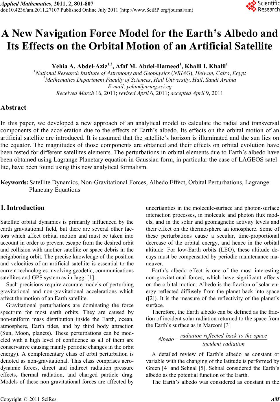
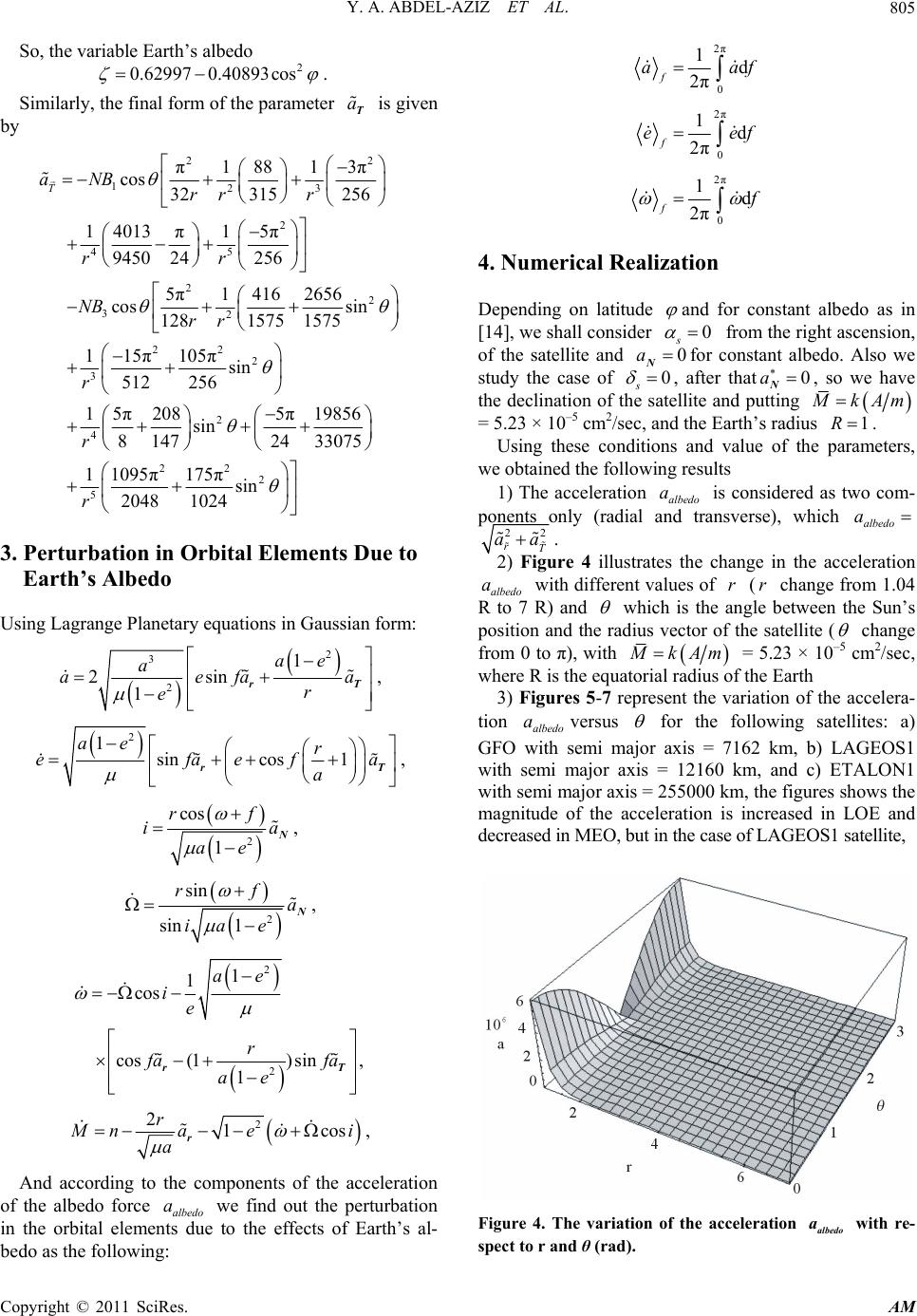
Figure 11. The Albedo perturbation in eccentricity for Star-
let satellite.
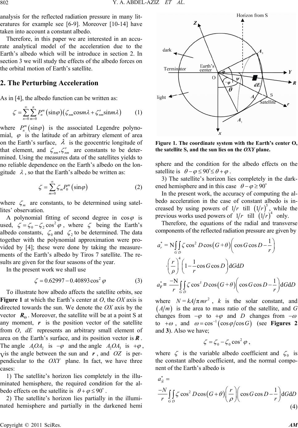
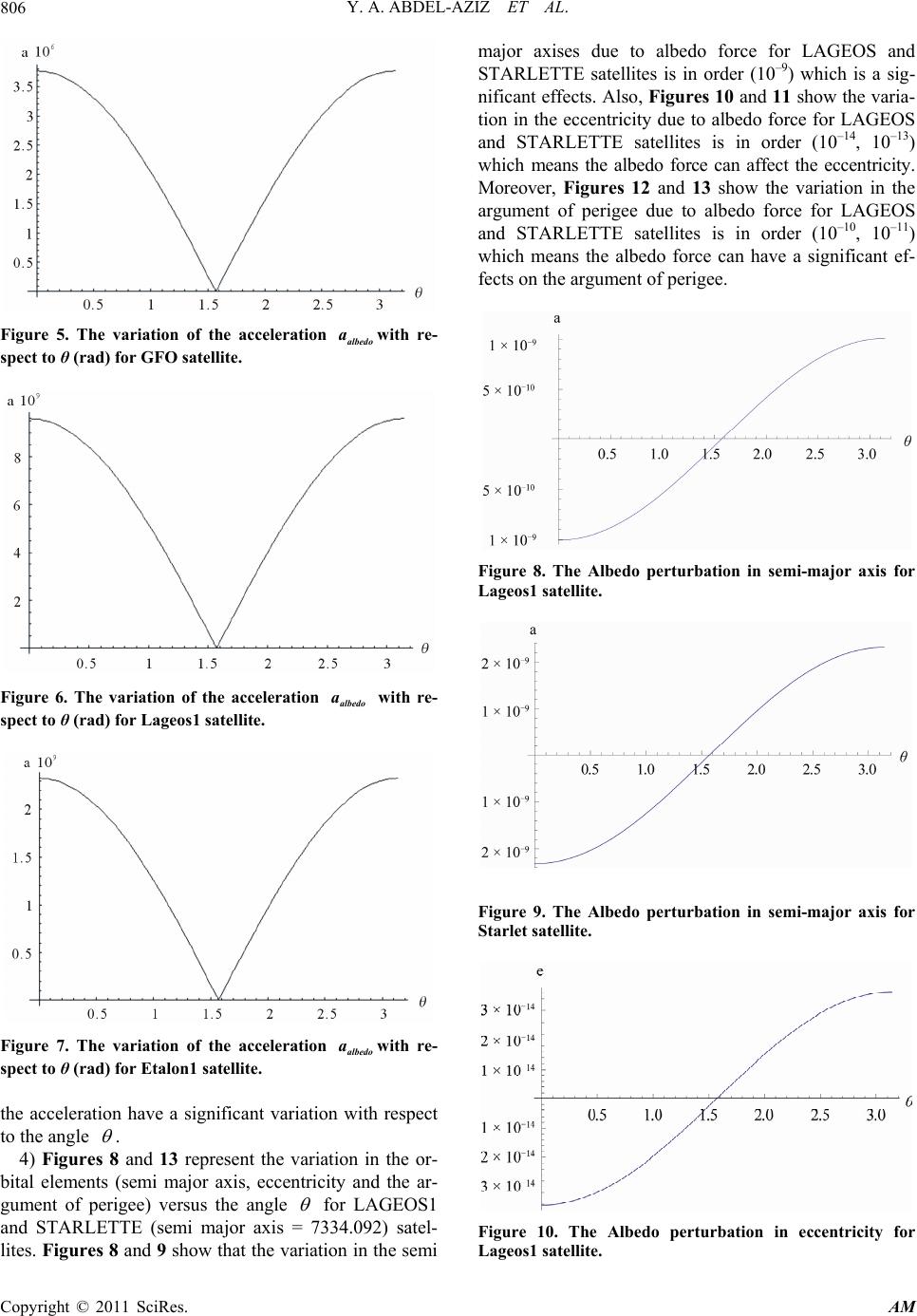
Figure 12. The Albedo per turbation in argument of perigee
for Lageos1 satellite.
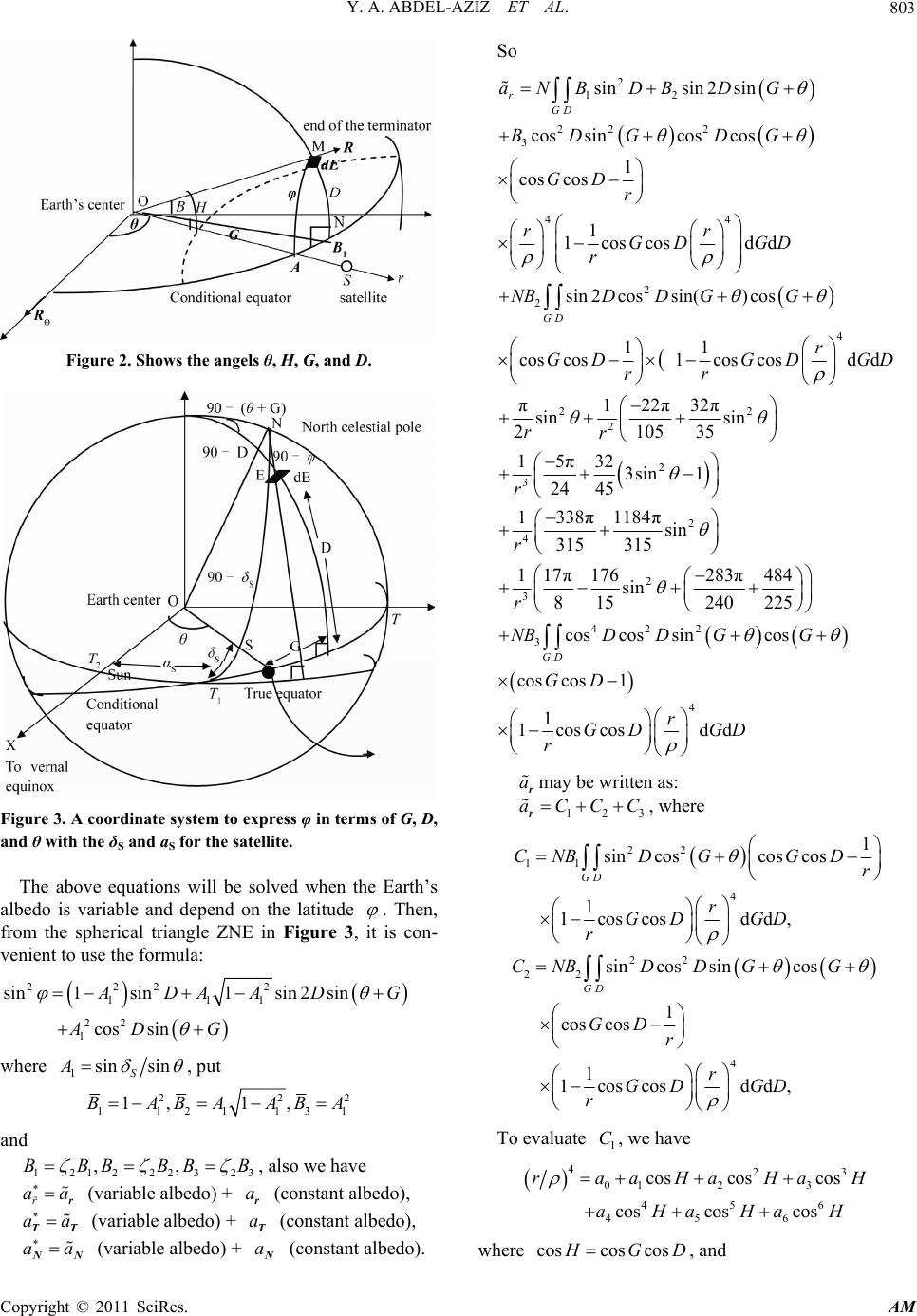
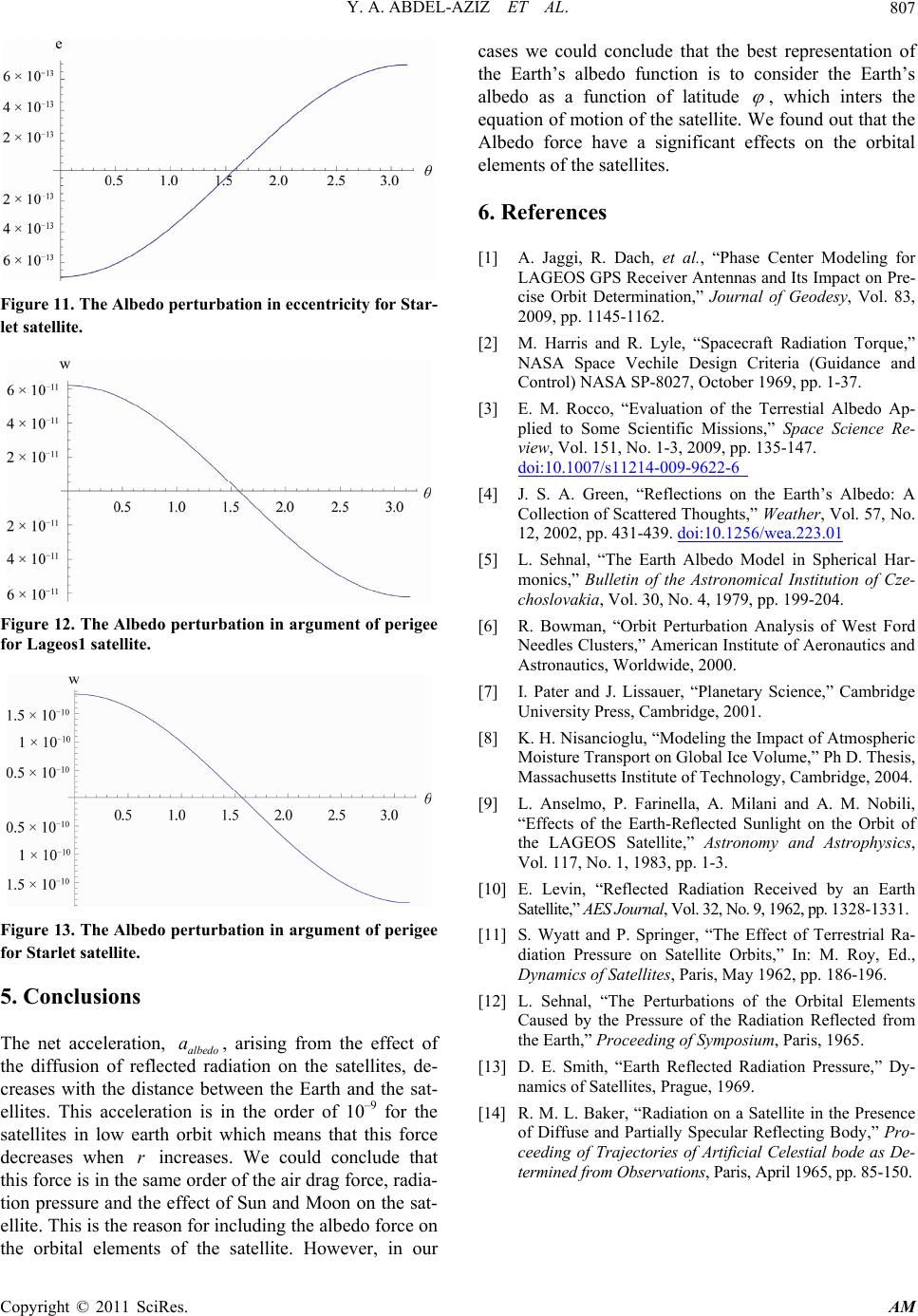
Figure 13. The Albedo per turbation in argument of perigee
for Starlet satellite.
n, , arising from the effect of
radiatio
5. Conclusions
The net acceleratio albedo a
the diffusion of reflectedn on the satellites, de-
creases with the distance between the Earth and the sat-
ellites. This acceleration is in the order of 10–9 for the
satellites in low earth orbit which means that this force
decreases when r increases. We could conclude that
this force is in the same order of the air drag force, radia-
tion pressure and the effect of Sun and Moon on the sat-
ellite. This is the reason for including the albedo force on
the orbital elements of the satellite. However, in our
cases we could conclude that the best representation of
the Earth’s albedo function is to consider the Earth’s
albedo as a function of latitude

, which inters the
equation of motion of the satellite. We found out that the
Albedo force have a significant effects on the orbital
elements of the satellites.
6. References
[1] A. Jaggi, R. D
LAGEOS GPS
ach, et al.ter Modeling for
Receiver Antenn Its Impact on Pre-
ignia (Guidance and
e Re-
, “Phase Cen
as and
Criter
cise Orbit Determination,” Journal of Geodesy, Vol. 83,
2009, pp. 1145-1162.
[2] M. Harris and R. Lyle, “Spacecraft Radiation Torque,”
NASA Space Vechile Des
Control) NASA SP-8027, October 1969, pp. 1-37.
[3] E. M. Rocco, “Evaluation of the Terrestial Albedo Ap-
plied to Some Scientific Missions,” Space Scienc
view, Vol. 151, No. 1-3, 2009, pp. 135-147.
doi:10.1007/s11214-009-9622-6
[4] J. S. A. Green, “Reflections on the Earth’s
Collection of Scattered Thoughts,”
Albedo: A
Weather, Vol. 57, No.
12, 2002, pp. 431-439. doi:10.1256/wea.223.01
[5] L. Sehnal, “The Earth Albedo Model in Spherical Har-
monics,” Bulletin of the Astronomical Institution of Cze-
utics and
lume,” Ph D. Thesis,
o. 9, 1962, pp. 1328-1331.
m
eflecting Body,” Pro-
choslovakia, Vol. 30, No. 4, 1979, pp. 199-204.
[6] R. Bowman, “Orbit Perturbation Analysis of West Ford
Needles Clusters,” American Institute of Aerona
Astronautics, Worldwide, 2000.
[7] I. Pater and J. Lissauer, “Planetary Science,” Cambridge
University Press, Cambridge, 2001.
[8] K. H. Nisancioglu, “Modeling the Impact of Atmospheric
Moisture Transport on Global Ice Vo
Massachusetts Institute of Technology, Cambridge, 2004.
[9] L. Anselmo, P. Farinella, A. Milani and A. M. Nobili,
“Effects of the Earth-Reflected Sunlight on the Orbit of
the LAGEOS Satellite,” Astronomy and Astrophysics,
Vol. 117, No. 1, 1983, pp. 1-3.
[10] E. Levin, “Reflected Radiation Received by an Earth
Satellite,” AES Journal, Vol. 32, N
[11] S. Wyatt and P. Springer, “The Effect of Terrestrial Ra-
diation Pressure on Satellite Orbits,” In: M. Roy, Ed.,
Dynamics of Satellites, Paris, May 1962, pp. 186-196.
[12] L. Sehnal, “The Perturbations of the Orbital Elements
Caused by the Pressure of the Radiation Reflected fro
the Earth,” Proceeding of Symposium, Paris, 1965.
[13] D. E. Smith, “Earth Reflected Radiation Pressure,” Dy-
namics of Satellites, Prague, 1969.
[14] R. M. L. Baker, “Radiation on a Satellite in the Presence
of Diffuse and Partially Specular R
ceeding of Trajectories of Artificial Celestial bode as De-
termined from Observations, Paris, April 1965, pp. 85-150.