Circuits and Systems, 2011, 2, 107-111
doi:10.4236/cs.2011.23016 Published Online July 2011 (http://www.SciRP.org/journal/cs)
An Improved Chirplet Transform and Its Application for
Harmonics Detection
Guo-Sheng Hu1, Feng-Feng Zhu2
1School of Computer, Shanghai Technical Institute of Electronics and Information, Shanghai, China
2School of Mathematics Science, South China University of Technology, Guangzhou, China
Received January 2, 2011; revised March 1, 2011; accepted March 8, 2011
Abstract
The chirplet transform is the generalization form of fast Fourier Transform, short-time Fourier transform,
and wavelet transform. It has the most flexible time frequency window and successfully used in practices.
However, the chirplet transform has not inherent inverse transform, and can not overcome the signal recon-
structing problem. In this paper, we proposed the improved chirplet transform (ICT) and constructed the in-
verse ICT. Finally, by simulating the harmonic voltages, the power of the improved chirplet transform are
illustrated for harmonic detection. The contours clearly showed the harmonic occurrence time and harmonic
duration.
Keywords: Harmonics, Improved Chirplet Transform (ICT), S-Transform, Time-Frequency Representation
(TFR)
1. Introduction
In many power quality analysis and disciplines, the con-
cept of a stationary time series is a mathematical ideali-
zation that is never realized and is not particularly useful
in the detection of power quality disturbances in power
systems. Although the Fourier transform of the entire
time series does contain information about the spectral
components in a time series, for a large class of practical
applications such as voltage signals in power systems,
this information is inadequate. So in the year of 1996,
Stockwell, Mansinha and Lowe presented a new S trans-
form that provides a joint time-frequency representation
(TFR) with frequency-dependent resolution [1] while, at
the same time, maintaining the direct relationship,
through time-averaging, with the Fourier spectrum. Sev-
eral have been proposed in the past; among them are the
Gabor transform [2], the related short-time Fourier trans-
forms [3], the continuous wavelet transform (CWT) [4],
and the bilinear class of time-frequency distributions
known as Cohen’s class [5], of which the Wigner distri-
bution [6] is a member. The S transform was defined as
following [1].
 

22
2π
2
,e
2π
tf jft
f
Sf htt




 


It is easy to prove that
ed.
.
(1)
 
,dSf Hf 

 
 (2)
where


H
f is the Fourier transform of


ht. It fol-
lows that


ht is exactly recoverable from


,Sf  .
Thus
 


2π
,de d.
jft
htS ff 
 
 
 (3)
The S-transforms have successfully been used in
power system disturbance detection and identification [7].
Another time-frequency representation, Chirplet trans-
form (CT), was defined by Mann Steven in 1992 [8].
 


2
2
2
2
1
,eed
2π
tb itqt
Cb htt





 

. (4)
From (4), it is easy to show that Chirplet transform is
an extension of Gabor transform, short-time Fourier
transform and continuous wavelet transform, furthermore,
the time-frequency window of CT is more flexible than
that of CWT. CT has been used successfully to classify
power quality disturbance (including voltage sag, voltage
swell, voltage interruption, and linear time-varying har-
monics and nonlinear time-varying harmonics) [9], de-
noise the motor fault signals [10], and detect slight fault
of electrical machines [11].

G.-S. HU ET AL.
108

,d.
However, CT does not satisfy basic characters (2) and
(3) and inconvenience in practical applications. So, in
this paper, we present an improved Chirplet transform
satisfying (2) and (3), moreover, the novel Chirplet
transform is an extension of the S-transform.
This paper is organized as follows. The improved
Chirplet transform is presented in Section 2, and the nu-
merical algorithm is introduced in Section 3; Several
simulated power quality harmonic waveforms are de-
tected and identified using the proposed method in Sec-
tion 4; Finally, The conclusions and references are given.
2. The Improved Chirplet Transform
Chirplet transform is considered as the “phase correc-
tion” of the CWT. The CWT of a function
is defined by [4]

,Wba

ht
 
,Wbahtwt bat



 (5)
where is a scaled replica of the fundamental
mother wavelet. The dilation a determines the “width” of
the wavelet and thus controls the resolution.
Along with (5), there exists an admissibility condition on
the mother wavelet [4] that must have
zero mean.

w

w

w

w
The improved chirplet transform of a function


ht
is defined as a CWT with a specific mother wavelet de-
fined as



22
2
22π
2
,ee
2π
tf iqiftqtfiq
wtf





. (6)
note that the frequency f and constant q.
The improved chirplet wavelet in (6) does not satisfy
the condition of zero mean for an admissible wavelet;
therefore, it is not strictly a CWT, Written out explicitly,
the improved chirplet transform is






22
2
22π
2
,
ee
2π
tbf iqifqtb
IC b f
fiq ht t






d.
.
(7)
It is obvious that Equation (7) degenerates to be an
S-transform as [1]. 0q
If the improved chirplet transform is indeed a repre-
sentation of the local spectrum, one would expect a sim-
ple operation of averaging the local spectra over time to
give the Fourier spectrum. It is shown as follows
 
,d
I
CbfbH f

 
 (8)
where

H
f

ht
is the Fourier transform of . It fol-
lows that is exactly recoverable from

ht



,
I
Cbf .
Thus
 


2π
,ded
ift
htICbf bf
 
 
 .
(9)
Proof: from








22 22
2
2
2
22
2
2
2
2
2
eede
1ed
2πed 2π.
tbf iqtbf iq
iq tb
u
u
bb
usetufiqb t
fiq
u
fiq
 

 

 


















d

we can get












22
2
22
2
22π
2
2
2π2
2π
,d
ee dd
2π
edee d
2π
ed ().
tbf iqiftqtb
tbf iqiqt b
ift
ift
IC b fb
fiq ht tb
fiq ht tb
httH f




 
 


 

 
 










.
Then (9) is the inverse of the above equation.
Alike FFT, STFT, WT, and CT, the improved chirplet
transform has the linear property. This is an advantage
over the bilinear class of time-frequency representations
(TFR’s). The presence of the cross terms makes it diffi-
cult to reliably estimate the signal. The improved chirplet
transform can be written as operations on the Fourier
spectrum


H
f of


ht
 
22
2
2π
2π
,e
ib fiq
IC b fHf


ed



 


 (11)
Proof:









22
2
22
2
2
22
2
22
2
2π
2π
2π
2π2π
2π
2
2π
222π
eed
()eee dd
eeded
ee
2π
(,
ib fiq
ift ib
fiq
fiq
tb fiq
ift
tbf iq
iftqtb
Hf
ht t
ht t
fiq ht t
IC b









 


  
 





 
  

 






  











).f
d
The discrete analog of (11) is used to compute the dis-
crete improved chirplet transform by taking advantage of
the efficiency of the Fast Fourier transform (FFT) and
the convolution theorem.

G.-S. HU ET AL.
109
3. The Discrete Improved Chirplet
Transform

1
0
1
,0 .
N
m
m
IC jTh
NNT





 (14)
with , and ,jm 0,1,2,,1nN

. The discrete im-
proved chirplet transform suffers the familiar problems
from sampling and finite length, giving rise to implicit
periodicity in the time and frequency domains. The dis-
crete inverse of the improved chirplet transforms (13)
and (14) is
Let


hkT , denote a discrete time
series corresponding to signal with a time sam-
pling interval of T. The discrete Fourier transform is
given by
0,1,2,,1kN

ht

2π
1
0
1e
ink
NN
k
n
HhkT
NT N





 .
N
(12)

2π
11
00
1,e.
j
nk
NN N
kj
n
hkTIC jT
NNT








 (15)
where . In the discrete case, the im-
proved chirplet transform is the projection of the vector
defined by the time series
0,1,2,,1n


hkT onto a spanning set of
vectors. The spanning vectors are not orthogonal, and the
elements of the improved chirplet transform are not in-
dependent. Each basis vector (of the Fourier transform)
is divided into localized vectors by an element-
by-element product with the N shifted Gaussians such
that the sum of these N localized vectors is the original
basis vector.
N
4. Examples
4.1. The Signal TFR Figure Using the Improved
Chirplet Transform
Using (11), the improved chirplet transform of a dis-
crete time series


hkT is given by (letting
f
nNT
and )

jT
2
2
2
2π2π
1
0
,e
mimj
NniqN
m
nmn
IC jTH
NT NT
 


 

 
 
e. (13)
Equations (7) and (9) are the improved chirplet transform
(ICT) for the time-frequency representation (TFR) and
its inverse ICT for the signal reconstruction. In the fol-
low figures, Figure 1(a) is the A-phase current signal of
the inductor motor with single phase grounding. Figure
2(b) shows the TFR of the A-phase current signal of the
motor using (7). The reconstruction signal using (9) is
illustrate in Figure 2(c). From Figure 1, we know (7)
and (9) are very effective for representing a time fre-
quency feature of a signal and reconstructing from TFR.
where , . For the , it is equal to
the constant defined as
0n

2
qqNT
0n
Figure 1. The motor A-phase current signal (a), its TFR (b), and the reconstructing signal.

110 G.-S. HU ET AL.
4.2. The harmonics Detection
Figures 2 and 3 demonstrate the class of time series for
which the improved chirplet transform would be useful;
they highlight the advantages of such an approach as
compared with other techniques.
Considering a simulating segment harmonic voltage
with zero initial phase as follows.






 


sin 25000.3
sin250 sin2 1500.3 0.6
sin 2500.20.61.4
sin2 50sin2 3501.41.7
sin 2501.72
pi tt
pi tpitt
ftpit tt
pi tpitt
pi tt
 
 


 

 

 



(16)
350 Hz
150 Hz 50 + 0.2t Hz
50 Hz
Figure 2. The simulating voltage with zero initial phase (a), and its ICT contour (b).
50 + 0.2t Hz
350 Hz
150 Hz
50 Hz
Figure 3. The simulating voltage with pi/3 initial phase (a), and its ICT contour (b).

G.-S. HU ET AL.
111
The voltage signal divided into 5 time segments. In the
first time interval, the voltage constrains only a fre-
quency: 50 Hz. At time 0.3, the voltage constrains an-
other harmonic: 150 Hz. In the time interval 0.6 1.4t

,
the voltage constrains a linear time changing harmonic.
Then at 1.4 s, the harmonic, 350 Hz, added to the signal.
Finally, the voltage retain normally at 1.7 s.
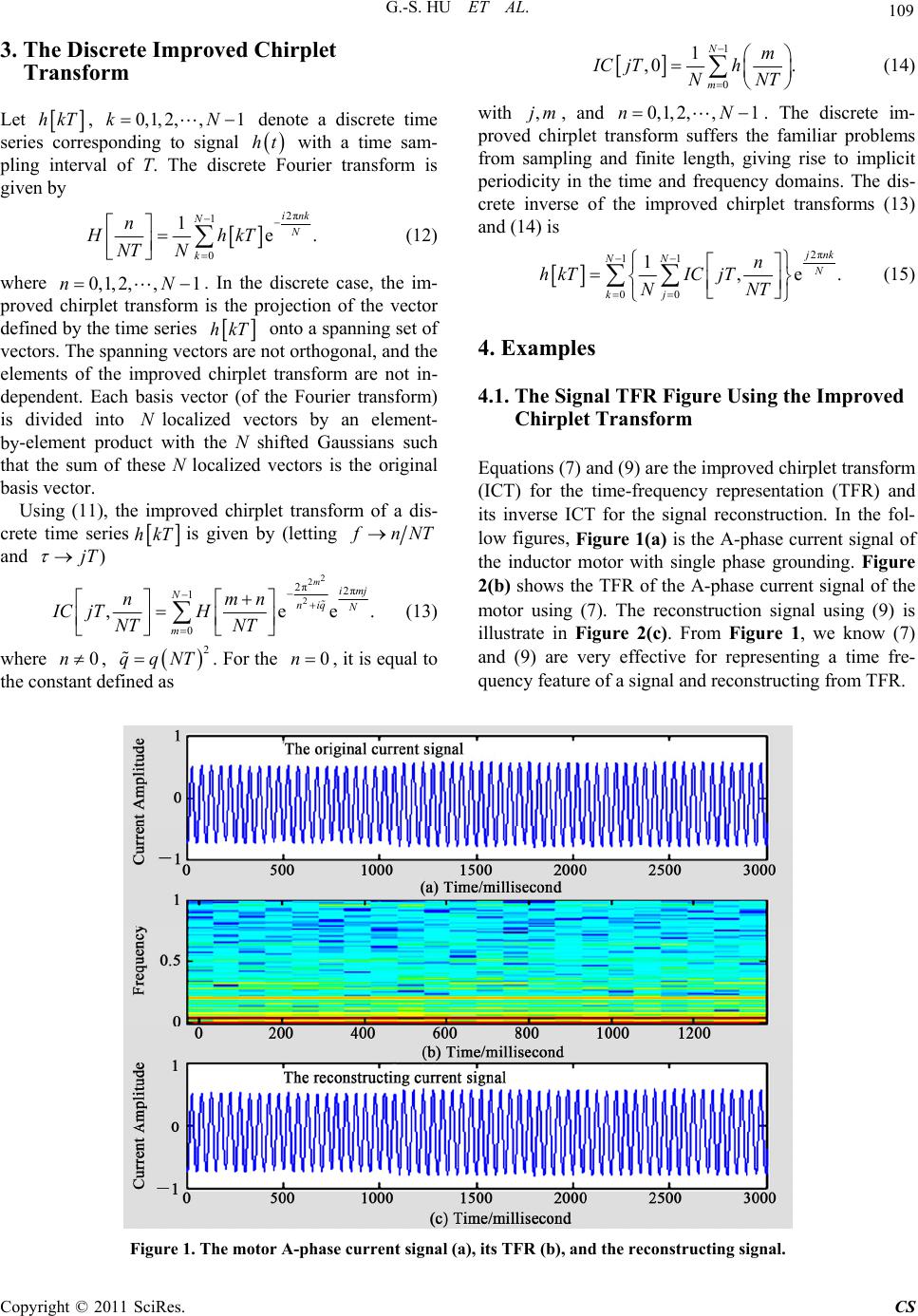
The sampling frequency is 1000 Hz. Figure 2 (a) is
the improved chirplet transform plot of (16). Figure 2(b)
is the contour plot of the signal (a) using (13) and (14).
Form Figure 2(b), we find the ICT contour illustrates the
work frequency 50 Hz, two harmonic frequency 150 Hz
and 350 Hz, and the linear time changing frequency 50 +
0.2 t Hz.
Moreover, the contour in Figure 2(b) clearly shows
the harmonic occurrence times and durations.
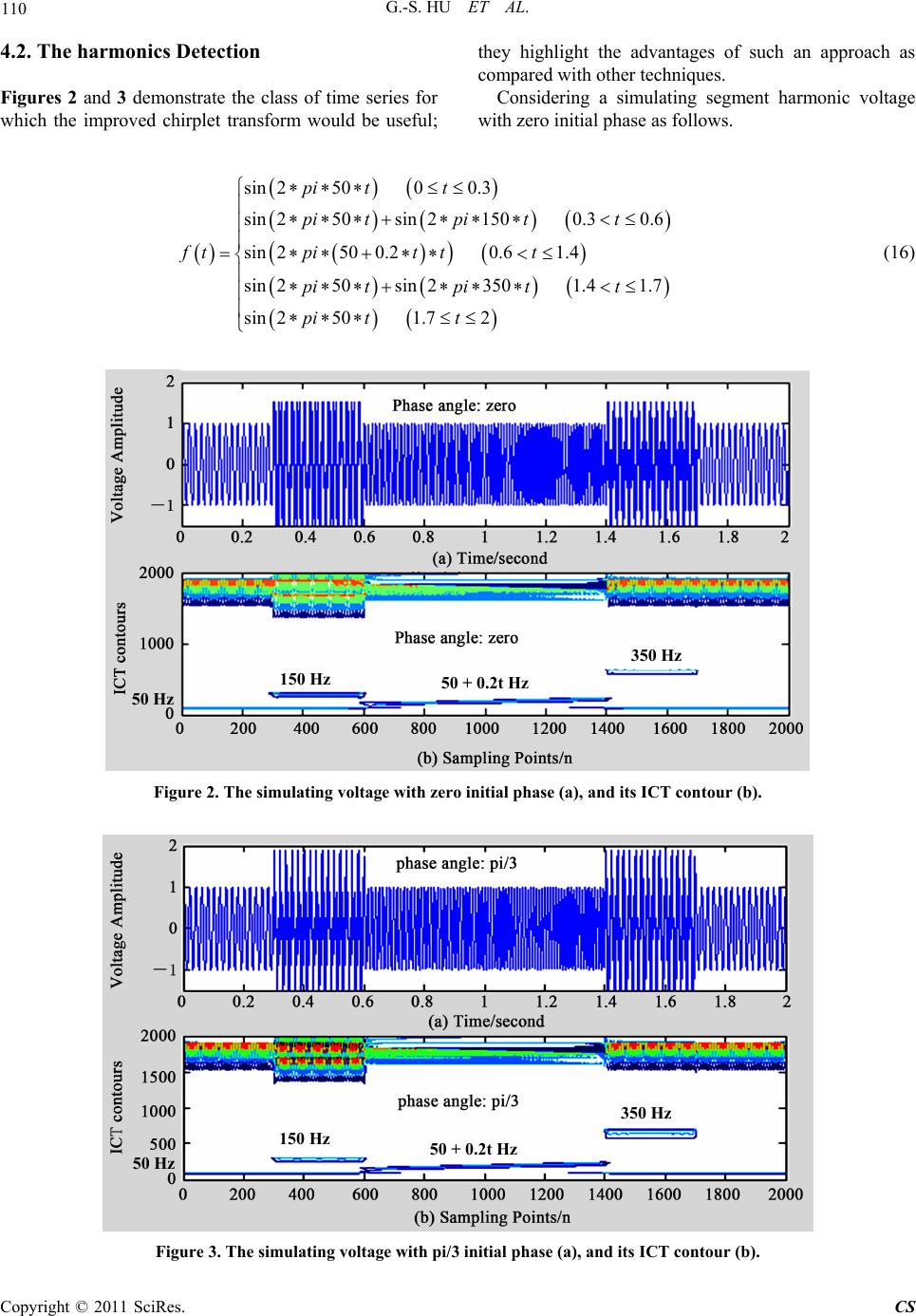
In order to investigate the influence of initial phase,
we modulating the above simulating voltage signal with
pi/3 phase. From Figure 3, we find that the initial phase
does not influence the harmonic detection.
5. Conclusions
The chirplet transform is the generalization form of fast
Fourier transform, short-time Fourier transform, and
wavelet transform. It has the most flexible time fre-
quency window and successfully used in practices.
However, the chirplet transform has not inherent recon-
structing formulae. So we proposed the improved chir-
plet transform (ICT) and constructed the inverse ICT.
Finally, the power of the improved chirplet transform is
apparent from the above examples.
6. References
[1] R. G. Stockwell, L. Mansinha and R. P. Lowe, “Location
of the Complex Spectrum: The S-Transform,” IEEE
Transactions on Signal Processing, Vol. 44, No. 4, 1996,
pp. 998-1001. doi:10.1109/78.492555
[2] D. Gabor, “Theory of Communication,” Journal of Insti-
tution of Electrical Engineers, Vol. 93, No. 3, 1946, pp.
429-457.
[3] R. N. Bracewell, “The Fourier Transform and Its Appli-
cations,” McGraw-Hill, New York, 1978.
[4] S. Mallat, “A Wavelet Tour of Signal Processing,” 2nd
Edition, Academic Press, Waltham, 2001.
[5] L. Cohen, “Time-Frequency Distributions—A Review,”
Proceedings of the IEEE, Vol. 77, No. 7, 1989, pp.
941-981. doi:10.1109/5.30749
[6] F. Hlawatsch and G. F. Boudreuax-Bartels, “Linear and
Quadratic Time-Frequency Signal Representations,” Pro-
ceedings of Signal Processing Magazine, Vol. 9, No. 2,
1992, pp. 21-67.
[7] M. V. Chilukur and P. K. Dash, “Multiresolution S-Trans-
form-Based Fuzzy Recognition System for Power Quality
Events,” IEEE Transactions on Power Delivery, Vol. 19,
No. 1, 2004, pp. 323-330.
doi:10.1109/TPWRD.2003.820180
[8] S. Mann and S. Haykin, “The Chirplet Transform: Physi-
cal Considerations,” IEEE Transactions on Signal Proc-
essing, 1995, Vol. 43, No. 11, pp. 2745-2761.
doi:10.1109/78.482123
[9] G.-S. Hu, F.-F. Zhu and Y.-J. Tu, “Power Quality Dis-
turbance Detection and Classification Using Chirplet
Transform,” Lecture Notes in Computer Science, Vol.
4247, 2006, pp. 34-41. doi:10.1007/11903697_5
[10] Z. Ren, G. S. Hu, W. Y. Huang and F. F. Zhu, “Motor
Fault Signals Denosing Based on Chirplet Transform,”
Transactions of China Electrotechnical Society, Vol. 17,
No. 3, 2002, pp. 59-62.
[11] G. S. Hu and F. F. Zhu, “Location of slight Fault in Elec-
tric Machine Using Trigonometric Spline Chirplet Trans-
forms,” Power System Technology, Vol. 27, No. 2, 2003,
pp. 28-31.