American Journal of Computational Mathematics, 2011, 1, 139-145
doi:10.4236/ajcm.2011.12015 Published Online June 2011 (http://www.scirp.org/journal/ajcm)
Thermal and Mechanical Modeling of Fluid and Heat Flow
in a Porous Metal Using Neural Networks for Application
as TPS in Space Vehicles
Prabhu. S. M.*, Abbas Soundarajan Mohadeen
Jhon Bosco college of Engineering Tiruvallur 631203
Mamallan inst of technology Sriperumbudur
Received May 9, 2011; revised May 31, 2011; accepted June 5, 2011
Abstract
This paper contains novel model using feedback neural networks for a work piece temperature prediction.
The heat and mass transfer in a porous metal workpiece which is heated by a fire gun is studied. The heat
flux distribution is determined by thermocouple connected on the workpiece at definite distances. The gun
work piece distance were also change and the temperature distribution and heat flux were determined. The
permeability’s were in range of 0.01 - 0.15. The ANN model parameters of the result output were simulated
using the ANN parameters the simulation was done using MATLAB 6.0® Neural Network Toolbox.
Keywords: Neyral Network, Porous Media, Prous Passages
1. Introduction
The heat and mass transfer in a porous metal workpiece
which is heated by a fire gun is studied. The heat flux
distribution in a workpiece due to effect of thermal spray
nozzle (uniform external heat source) causing high radia-
tion conduction and convection transfer in the workpiece.
The flame gun was kept at various distance and the effect
of the source studied for the radiation and convection.
This work mainly deals with the studies on heat flux and
temperature prediction in a metal workpiece subjected to
firing gun (fired using mixture of oxygen and acetylene
gas) generally used for gas cutting and welding opera-
tions
Studies on Flow and transport at interface between a
porous medium and clear fluid have been studied widely.
Fauchius, Vandelle and others [1] studied the mecha-
nisms and models for Thermal spraying. Sampath and
Jiang [2] discussed the procedures for computing design
parameters in Substrate temperature spray coatings. Pop
[3] did studies on modeling of heat flow in a porous cav-
ity. Lai [4] studied the effect of Non-Darcy Convection
in the free surface of a porous media. In this paper a
gener- alized treatment of convection force and the effect
of free surface hydrodynamics on the heat transfer is
dealt with. A novel model incorporating computation of
local and average heat flux has been discussed. Ras [5,6]
did studies on the free surface convection while others
including Lai [4] studied the Forced convection on the
surface of porous layer. Pop and Postelnicu [7] discu ssed
on the effect of heat generation effect on the layers in
porous media.
Flow and transport at interface between a porous me-
dium and clear fluid is of importance in heat transfer in
porous enclosures and extended surfaces. The mecha-
nisms that contribute to the enhanced heat transfer in-
clude heat conduction in the metal foam matrix (whose
conductivity is always higher by several orders of mag-
nitude .The well known Darcy’s law is based on a bal-
ance between the present gradient and the viscous forces
and breaks down for high velocities when inertia terms
are no longer negligible. Here we present numerical and
experimental results for buoyancy induced flow in a high
porosity metal foam
The Associative Neural network (ASNN) is an
extension of the ANN that goes beyond a simple/
weighted average of different models. Associative
Neural network represents a combinatio n of an ensemble
of feed-forward neural networks and the k-nearest nei-
ghbor technique. It uses the correlation between ensem-
ble responses as a measure of distance amid the analyzed
cases for the ANN. This corrects the bias of the neural

PRABHU. S. M. ET AL. 140
network ensemble. An associative neural network has a
memory that can coincide with the training set. If new
data becomes available, the network instantly improves
its predictive ability and provides data approximation
(self-learn the data) without a need to retrain the en-
semble. Another important feature of ASNN is the
possibility to interpret neural network results by analysis
of correlations between data cases in the space of models.
BAM (binary associative memory) is the recurrent
memory achieved by the exemplar on being trained by
standard inputs prior to its deployment for modeling and
simulation applications
2. Experimental Methods:
The heat flux distribution is determined by thermocouple
connected on the workpiece at definite distances. The
gun work piece distance were also changed and the tem-
perature distribution and heat flux were determined.
Cu-Ni Thermocouples were attached on the surface of
the workpiece. The flame was generated by acetylene
and oxygen gasses as in gas welding process, the flame
was kept at distances from 5 cm to 20 cm and the heat
flux distrib ut i o n st udi ed.
During a typical experimental run the powers were
varied to achieve different base late temperature and
hence Rayleigh numbers. Due to temperature constraints
the parameters of the heat input were restricted to maxi-
mum base plate temperature of 80*c a metal foam sam-
ple heated from above .
The foam sample is saturated with & surrounded by a
fluid, which extends a distance 1
s
in
x
direction and
2
s
in y direction.
The steady two dimensional equations for the fluid
saturated porous medium & for the clear fluid region
outside the metal foam are written separately as shown
below.
The Flow in a Square Pore cavity is modeled using the
continuity and energy equations using a square computa-
tional grid with velocity and temperatur e boundaries.
The continuity and energy equations are given by
0
uv
r



 (1)
2
222
1uu vvuT
a
rr r




 
 

  

(2)
where volumetric heat sources

, , ryz represents the
contribution of frictional heating. The parameters
p
C

& e k may depend on y & z but remain independ-
ent of r. More importantly the contribution of axial
conduction deferred to the subsequent is neglected,
hence Equation (4 ) red uces

22 22
22 p
uvuv
uva uv
rr kc r

 






 (3)

0
1
TT
uv
rr
TT
Q
rr





 
 
 
 

 
(4)
where the Heat generation number d Q is given by
2
0"
()
ref
f
fpf hc
Lq
QCTT

 (4a)
The governing equations are scaled on basis of fluid
Raleigh number as in the case of viscous fluid (inde-
pendent of permeability) instead of modified Raleigh’s
number. The scaling is introduced to study the effective
change in values of individual matrix & fluid parameters
(6). Finite element method is used for prediction of pa-
rameters. A suitable grid scheme with iso-parametric,
quadrilateral elements is used for stability of numerical
solution, all the elements are containing 8 nodes, one at
each corner and one at midpoint of each of the sides. All
nodes are given velocity & temperature boundaries and
corners of the grid pressure boundaries. This is an ac-
cepted practice given by Taylor (2). For depicting the
variation in pressure by the shape function i
M
of one
order less than shape function i
N defined for velocities
and temperature.
2.1. Direct Problem:
2
pTTT
Ckr
rrrz


 


 
(5)
 
, t>0 0,
kT qrtrR zH
z



 (5a)

00 0.
Tzr R
n

 (5b)


0 0 at 0,TT trR (5c)
2.2. Sensitivity Problem
2
pTTT
Ckr
rrrz






 
(6)
 
, >0 0, =
kT qrt trRzH
z

 (7)

0, 0,0.
Tzr R
n

 (8)

PRABHU. S. M. ET AL. 141
2.3. Adjoint Problem
  
2
,,;
ms msms
J
qrTrztqYt

 

(9)
where (, , , )
ms ms
Trztq is the temperature calculated at
the measuring points (rms) through the direct problem
Equations 5 & (5a)-(c), Yms(t) is measured temperature
and the subscript ms denotes the thermocouple n umber.
The adjoint problem is obtained by introducing the
Lagrange multiplier

, , rzt  into the direct problem
equations and by integrating over the spatial and then
over the temporal domain as follows.
For the region (0, )rR,(0, )zH




3
, , , at t>0
p
w
ms
Tr
Ck
ttrz
rr
Trztq Ytzz










 


(10)

0, 0, =0., z=0,zrR H
n
 
 (11)


0 0., 0
f
ttrRz H    (12)
where

  is the Dirac delta function. It is required
for solving the adjoint equations with the end condition
at time
f
tt, one should first proceed with variable
change
f
tt

 , The adjoint problem becomes an ini-
tial value problem in

via the transformation.
Step size and Gradient
The iterative equation for determining

, , qrzt can
be given by
 
11
,,(,)
nn n
qrtqrt Prt 

 (13)
where the superscript n denotes the iteration number
and n

is the search stepsize defined by
 

00
2
00
, , ;
, , ;
HHnmz msms
n
HRn mz ms
Tr ztqYtdrdt
rTrztq drdt



 

 (14)
and the descendin g direct i o n n
P is estimated by
 
1
, , , ,
nnnn
p rztprzt 

 (15)
Where 1n, 10
 . General definition of

is
given by
  

1
2
1
,
n nnn
n
qqq
q







(16)
where  represents the norm and (.,.) the scalar prod-
uct.
Time stepsize and algorithm stop criterion
The stopping criterion is satisfied when the Fourier
Table 1. Properties of workpiece (Cu).
Thermal conductivity k=396w/m·c
p
C389J/kg·c
Density = 8900kg/m3
Table 1a. Artificial Neural Network (ANN) variable de-
scription.
CategoryParameter Lower
limit Upper limit Neuron number
D gun workpiece dis-
tance 30 100 1
t-preheating time
s
0 10 1
1
YFirstthermocouple
temperature
10 60 3
2
Ysecondthermocouple
temperature 10 65 2
3
Ythirdthermocouple
temperature 10 60 5
Input pat-
tern
radial position mm 0 50 4
Output
pattern q-heat flux Mw/sqm 0 1.2 1
number (o
F
) satisfies the condition
0.05
optp
kt
FCH


 (17)
where 0.028
o
F

,

is the time step, and tp
H
is the
location of thermocouples to the surface in front of the
flame ,according to parameters listed in Table 1.
Since the Fourier number satisfies Equation (17),the
increase of measuring errors is weak and few obvious
noisy signals can be captured. In this study, 0.5st


has been considered for the time step according to the
limit of data acquisition system. If the problem contains
no noisy signals, the general stopping criterion condition
is expressed by


Jq


(18)
Where

is specified stopping criterion. But the
measurement precision of data

acquisition is about
10-3. Hence it should not be reasonable to expect the
functional Equation (9) to be equal to zero. A small value
of 0.002


is chosen for above criterion
Algorithm for CGM method
The algorithm for Conjugate gradient method (CGM) is
given belo w.
1) Select an initial guess

,
n
qrt. generally equal to
zero.
2) Calculate the direct problem, Equations (1)-(4), ob-
tain the solution


, , ;
n
ms ms
Trztq .
3) Decide if the stopping criterion Equation (18) is
satisfied. If yes go to step (6), otherwise continue.
4) Solve the adjoint problem. Equations (10)-(12)
[note: 1 =(t )t


in place of t], calculate the conjugate

PRABHU. S. M. ET AL. 142
Table 2. ANN output results of parameters.
Time t secs r
y p y t;
E
kl
I
D m 1
Y m 2 Y m 3 Y m Radial posn heat flux q MW/sqm
8 0.87 0.54 0.05 0.51 0.056 0.028 0.039 0.06 20 0.7
9 0.92 0.63 0.07 0.73 0.082 0.035 0.054 0.064 22 0.81
10 1.01 0.78 0.095 0.81 0.093 0.055 0.07 0.073 26 0.98
12 1.21 0.91 0.11 0.96 0.098 0.07 0.085 0.082 29 1.03
Table 3. Computation of flux parameters using CGM.
Time t secs .n(cm)

n
Pr, z, t.

n+1
qr, t
f
T T

f
=T T 

t
o
E

.
q o
F
d
Q
2 1.83 0.628 340 280 60 0.15 1.5 2.43 0.185 0.003
4 1.84 0.651 347 284 63 0.173 1.48 2.45 0.21 0.0034
2
6 1.91 0.731 378 293 68 0.18 1.54 2.63 0.27 0.0041
2 1.41 0.78 390 297 72 0.21 1.64 2.71 0.32 0.0046
4 1.63 0.82 410 302 78 0.28 1.81 2.91 0.45 0.0047 4
6 1.73 0.87 412 308 81 0.32 1.92 3.12 0.51 0.0049
2 1.45 0.81 402 304 74 0.23 1.71 2.8 0.41 0.005
4 1.71 0.92 408 307 76.3 0.28 1.81 2.9 0.43 0.0051 6
6 1.81 1.02 415 308 77.4 0.41 1.93 3.2 0.48 0.0053
2 1.84 1.08 418 312 79 0.48 2.01 3.43 0.52 0.0054
4 1.86 1.13 421 315 81 0.51 2.11 3.51 0.58 0.0056 8
6 1.91 1.31 428 321 85 0.61 2.33 3.81 0.7 0.0058
coefficient n

, Equation (19) and the direction of de-
scendent n p Equa t i on (1 8).
5) Solve the sensitivity problem Equations (5)-(8),
calculate the stepsize n

from the nth to the (1n

)st
iteration, Equation (17) and calculate a new vector 1n q

.
Go to step 2.
6) The iteration is terminated.
3. A Neural Computational Procedure
The heat flux calculated by solving the inverse problem
was correlated to the workpiece temperature and other
parameters with the aid of an artificial neural network
(ANN). Such a structure considers three main categories.
1) The processing and the experiment design parame-
ters with aid of an artificial neural network (ANN). Such
a structure considers following types.
2) The processing and experiment design parameter as
an input (1) pattern. These were the gun workpiece dis-
tance, the preheating time, the thermocouple tempera-
tures and radial position.
3) The heat flux as an output (O) unit calculated using
CGM.
4) An intermediate structure called hidden layers, en-
coding the corr elat i ons bet ween I/O patterns.
Each of the ANN types is defined by a set of neurons
playing role of simple processing elements as in Table
1a. A neuron has ability to receive a sum of numbers
from other neurons and to emit a signal number toward
other neurons accor ding to
11kijk ij
I
WO

(19)
where 1k
I
is input of neuron l from layer k, ij O is
output of neuron j from layer; 1ijk
W is called the weight
relating neuron j and neuron 1 and this corresponds to
neuron strength




1,,( , )2.351.450.628 nnn
qrtqrt Prt 
 
from (16)







1
22
1
,1.2 0.730.243
1.43
nnnn
n
qq q
q
 








00.05 /
396 1.5
0.8850.05
8900389 0.0021
tp
ptp
kt
FtH
CH






from (14)



1
, , , ,
1.21.50.431.83
nnnn
P rztPrzt 



from (4a) we h a ve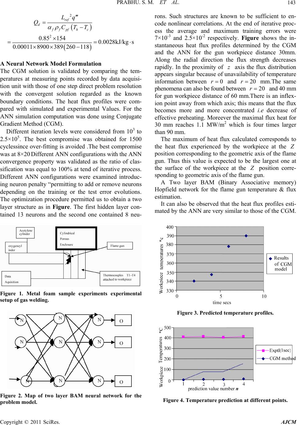

PRABHU. S. M. ET AL. 143


2
2
0.85 1540.0028kJ/kg s
0.000118900389 260118
ref
dffpf hc
Lq
QCTT





 
A Neural Networ k Mo del F ormulation
The CGM solution is validated by comparing the tem-
peratures at measuring points recorded by data acquisi-
tion unit with those of one step direct problem resolution
with the convergent solution regarded as the known
boundary conditions. The heat flux profiles were com-
pared with simulated and experimental Values. For the
ANN simulation computation was done using Conjugate
Gradient Method (CGM).
Different iteration levels were considered from 103 to
2.5×105. The best compromise was obtained for 1500
cyclessince over-fitting is avoided .The best compromise
was at 8×20 Different ANN configurations with the ANN
convergence property was validated as the ratio of clas-
sification was equal to 100% at tend of iterative process.
Different ANN configurations were examined introduc-
ing neuron penalty “permitting to add or remove neurons
depending on the training or the test error evolutions.
The optimization procedure permitted us to obtain a two
layer structure as in Figure. The first hidden layer con-
tained 13 neurons and the second one contained 8 neu-
Figure 1. Metal foam sample experiments experimental
setup of gas welding.
Figure 2. Map of two layer BAM neural network for the
problem model.
rons. Such structures are known to be sufficient to en-
code nonlinear correlations. At the end of iterative proc-
ess the average and maximum training errors were
7×10-3 and 2.5×10-2 respectively. Figure shows the in-
stantaneous heat flux profiles determined by the CGM
and the ANN for the gun workpiece distance 30mm.
Along the radial direction the flux strength decreases
rapidly. In the proximity of z axis the flux distribution
appears singular because of unavailab ility of temperature
information between 0r

and 20r mm.The same
phenomena can also be found between 20r and 40 mm
for gun workpiece distance of 60 mm.There is an inflex-
ion point away from which axis; this means that th e flux
becomes more and more concentrated i.e decrease of
effective preheating. Moreever the maximal flux heat for
30 mm reaches 1.1 MW/m2 which is four times larger
than 90 mm.
The maximum of heat flux calculated corresponds to
the heat flux experienced by the workpiece at the
Z
position corresp onding to the geometric axis of the flame
gun. Thus this value is expected to be the largest one at
the surface of the workpiece at the
Z
position corre-
sponding to geometric axis of the flame gun.
A Two layer BAM (Binary Associative memory)
Hopfield network for the flame gun temperature & flux
estimation.
It can also be observed that the heat flux profiles esti-
mated by the ANN are very similar to those of the CGM.
Figure 3. Predicted temperature profiles.
Figure 4. Temperature prediction at different points.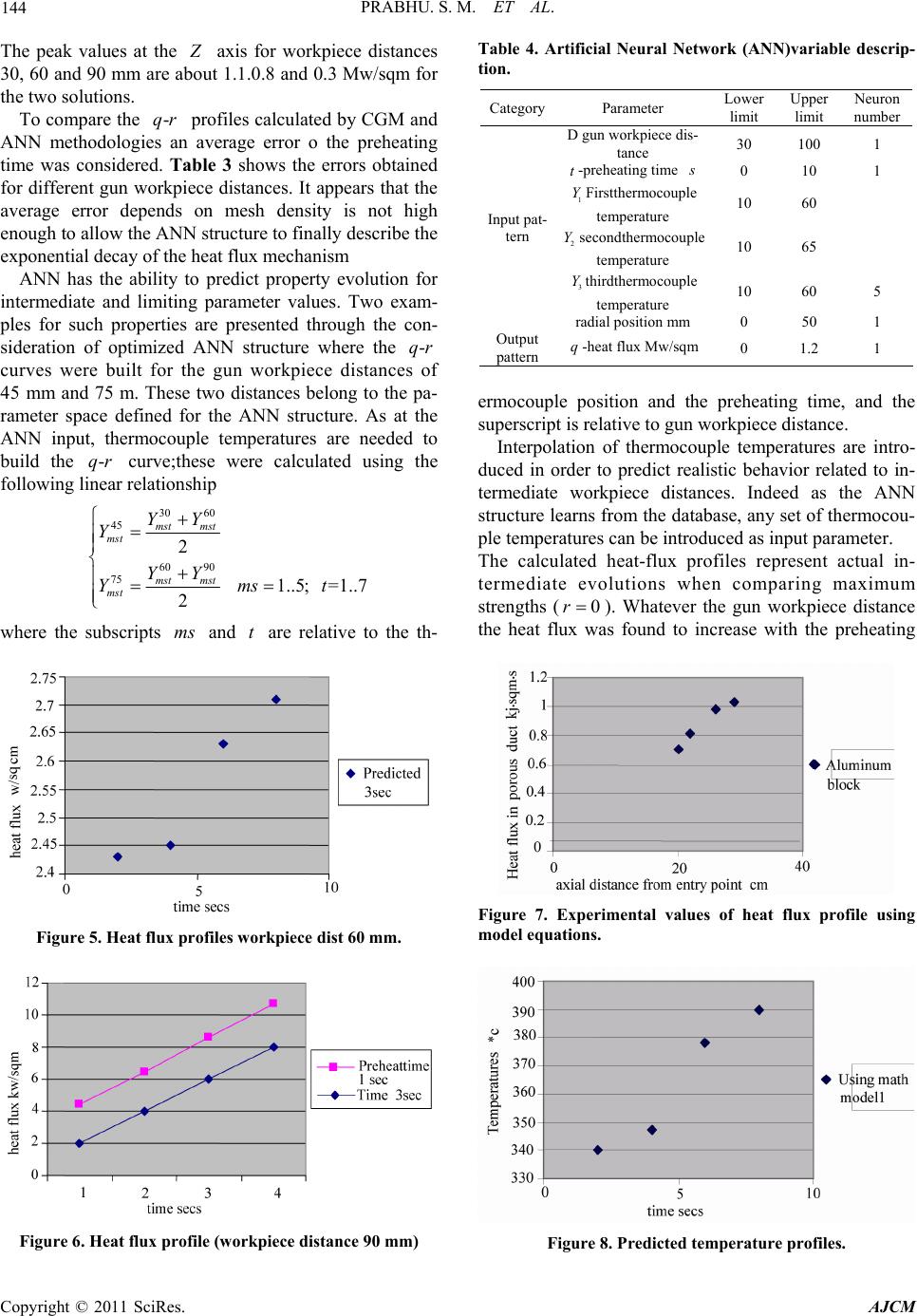

PRABHU. S. M. ET AL. 144
The peak values at the
Z
axis for workpiece distances
30, 60 and 90 mm are about 1.1.0.8 and 0.3 Mw/sqm for
the two solution s .
To compare the -qr profiles calculated by CGM and
ANN methodologies an average error o the preheating
time was considered. Table 3 shows the errors obtained
for different gun workpiece distances. It appears that the
average error depends on mesh density is not high
enough to allow the ANN structure to finally describe the
exponential decay of the heat flux m echanism
ANN has the ability to predict property evolution for
intermediate and limiting parameter values. Two exam-
ples for such properties are presented through the con-
sideration of optimized ANN structure where the -qr
curves were built for the gun workpiece distances of
45 mm and 75 m. These two distances belong to the pa-
rameter space defined for the ANN structure. As at the
ANN input, thermocouple temperatures are needed to
build the -qr curve;these were calculated using the
following linear relationship
30 60
45
60 90
75
2
1..5; =1..7
2
mst mst
mst
mst mst
mst
YY
Y
YY
Ymst








where the subscripts ms and t are relative to the th-
Figure 5. Heat flux profiles workpiece dist 60 mm.
Figure 6. Heat flux profile (workpiece distance 90 mm)
Table 4. Artificial Neural Network (ANN)variable descrip-
tion.
CategoryParameter Lower
limit Upper limit Neuron number
D gun workpiece dis-
tance 30 100 1
t-preheating time
s
0 10 1
1
YFirstthermocouple
temperature
10 60
2
Ysecondthermocouple
temperature 10 65
3
Ythirdthermocouple
temperature 10 60 5
Input pat-
tern
radial position mm 0 50 1
Output
pattern q-heat flux Mw/sqm 0 1.2 1
ermocouple position and the preheating time, and the
superscript is relative to gun workpiece distance.
Interpolation of thermocouple temperatures are intro-
duced in order to predict realistic behavior related to in-
termediate workpiece distances. Indeed as the ANN
structure learns from the database, any set of thermocou-
ple temperatures can be introduced as input parameter.
The calculated heat-flux profiles represent actual in-
termediate evolutions when comparing maximum
strengths (0r

). Whatever the gun workpiece distance
the heat flux was found to increase with the preheating
Figure 7. Experimental values of heat flux profile using
model equations.
Figure 8. Predicted temperature profiles.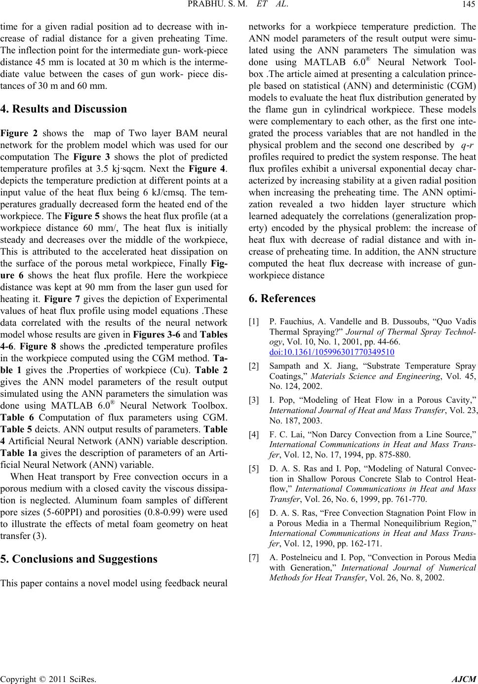

PRABHU. S. M. ET AL. 145
time for a given radial position ad to decrease with in-
crease of radial distance for a given preheating Time.
The inflection point for the intermediate gun- work-piece
distance 45 mm is located at 30 m which is the interme-
diate value between the cases of gun work- piece dis-
tances of 30 m and 60 mm.
4. Results and Discussion
Figure 2 shows the map of Two layer BAM neural
network for the problem model which was used for our
computation The Figure 3 shows the plot of predicted
temperature profiles at 3.5 kj·sqcm. Next the Figure 4.
depicts the temperature prediction at different points at a
input value of the heat flux being 6 kJ/cmsq. The tem-
peratures gradually decreased form the heated end of the
workpiece. The Figure 5 shows the heat flux profile (at a
workpiece distance 60 mm/, The heat flux is initially
steady and decreases over the middle of the workpiece,
This is attributed to the accelerated heat dissipation on
the surface of the porous metal workpiece, Finally Fig-
ure 6 shows the heat flux profile. Here the workpiece
distance was kept at 90 mm from the laser gun used for
heating it. Figure 7 gives the depiction of Experimental
values of heat flux profile using model equations .These
data correlated with the results of the neural network
model whose results are given in Figures 3-6 and Tables
4-6. Figure 8 shows the .predicted temperature profiles
in the workpiece computed using the CGM method. Ta-
ble 1 gives the .Properties of workpiece (Cu). Table 2
gives the ANN model parameters of the result output
simulated using the ANN parameters the simulation was
done using MATLAB 6.0® Neural Network Toolbox.
Table 6 Computation of flux parameters using CGM.
Table 5 deicts. ANN output results of parameters. Table
4 Artificial Neural Network (ANN) variable description.
Table 1a gives the description of parameters of an Arti-
ficial Neural Network (ANN) variable.
When Heat transport by Free convection occurs in a
porous medium with a closed cavity the viscous dissipa-
tion is neglected. Aluminum foam samples of different
pore sizes (5-60PPI) and porosities (0.8-0.99) were used
to illustrate the effects of metal foam geometry on heat
transfer (3).
5. Conclusions and Suggestions
This paper contains a novel model using feedback neural
networks for a workpiece temperature prediction. The
ANN model parameters of the result output were simu-
lated using the ANN parameters The simulation was
done using MATLAB 6.0® Neural Network Tool-
box .The article aimed at presenting a calculation prince-
ple based on statistical (ANN) and deterministic (CGM)
models to evaluate the heat flux distribution generated by
the flame gun in cylindrical workpiece. These models
were complementary to each other, as the first one inte-
grated the process variables that are not handled in the
physical problem and the second one described by -qr
profiles required to predict the system response. The heat
flux profiles exhibit a universal exponential decay char-
acterized by increasing stability at a given radial position
when increasing the preheating time. The ANN optimi-
zation revealed a two hidden layer structure which
learned adequately the correlations (generalization prop-
erty) encoded by the physical problem: the increase of
heat flux with decrease of radial distance and with in-
crease of preheating time. In addition , the ANN structure
computed the heat flux decrease with increase of gun-
workpiece distance
6. References
[1] P. Fauchius, A. Vandelle and B. Dussoubs, “Quo Vadis
Thermal Spraying?” Journal of Thermal Spray Technol-
ogy, Vol. 10, No. 1, 2001, pp. 44-66.
doi:10.1361/105996301770349510
[2] Sampath and X. Jiang, “Substrate Temperature Spray
Coatings,” Materials Science and Engineering, Vol. 45,
No. 124, 2002.
[3] I. Pop, “Modeling of Heat Flow in a Porous Cavity,”
International Journal of Heat and Mass Transfer, Vol. 23,
No. 187, 2003.
[4] F. C. Lai, “Non Darcy Convection from a Line Source,”
International Communications in Heat and Mass Trans-
fer, Vol. 12, No. 17, 1994, pp. 875-880.
[5] D. A. S. Ras and I. Pop, “Modeling of Natural Convec-
tion in Shallow Porous Concrete Slab to Control Heat-
flow,” International Communications in Heat and Mass
Transfer, Vol. 26, No. 6, 1999, pp. 761-770.
[6] D. A. S. Ras, “Free Convection Stagnation Point Flow in
a Porous Media in a Thermal Nonequilibrium Region,”
International Communications in Heat and Mass Trans-
fer, Vol. 12, 1990, pp. 162-171.
[7] A. Postelneicu and I. Pop, “Convection in Porous Media
with Generation,” International Journal of Numerical
Methods for Heat Transfer, Vol. 26, No. 8, 2002.