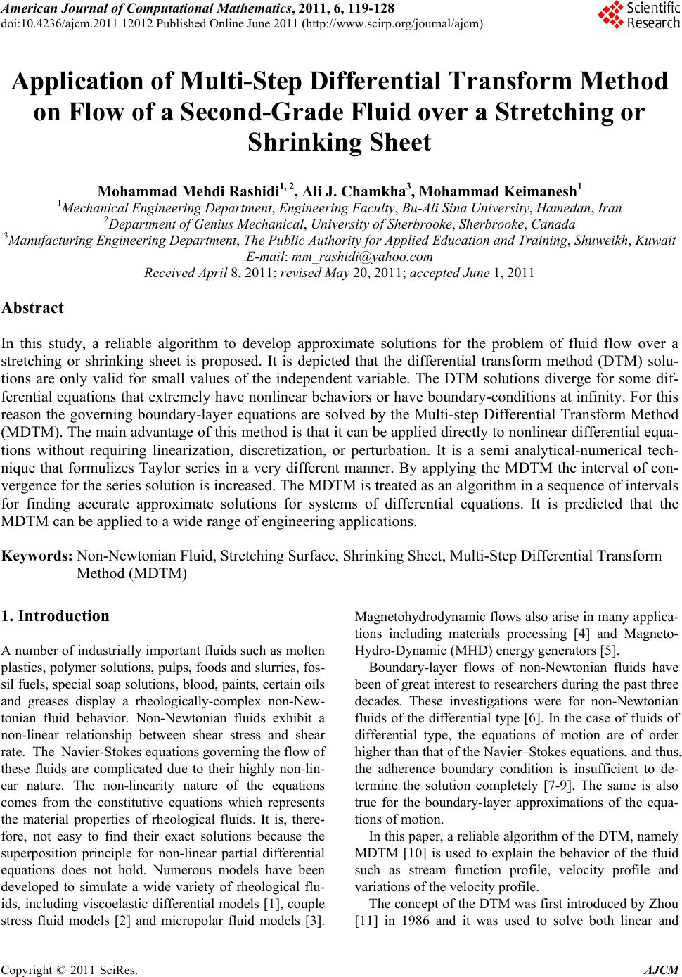American Journal of Computational Mathematics, 2011, 6, 119-128
doi:10.4236/ajcm.2011.12012 Published Online June 2011 (http://www.scirp.org/journal/ajcm)
Application of Multi-Step Differential Transform Method
on Flow of a Second-Grade Fluid over a Stretching or
Shrinking Sheet
Mohammad Mehdi Rashidi1, 2, Ali J. Chamkha3, Mohammad Keimanesh1
1Mechanical Engineering Department, Engineering Faculty, Bu-Ali Sina University, Hamedan, Iran
2Department of Genius Mechanical, University of Sherbrooke, Sherbrooke, Canada
3Manufacturing Engineering Department, The Public Authority for Applied Education and Training, S huw ei kh, Kuwait
Received April 8, 2011; revised May 20, 2011; accepted June 1, 2011
Abstract
In this study, a reliable algorithm to develop approximate solutions for the problem of fluid flow over a
stretching or shrinking sheet is proposed. It is depicted that the differential transform method (DTM) solu-
tions are only valid for small values of the independent variable. The DTM solutions diverge for some dif-
ferential equations that extremely have nonlinear behaviors or have boundary-conditions at infinity. For this
reason the governing boundary-layer equations are solved by the Multi-step Differential Transform Method
(MDTM). The main advantage of this method is that it can be applied directly to nonlinear differential equa-
tions without requiring linearization, discretization, or perturbation. It is a semi analytical-numerical tech-
nique that formulizes Taylor series in a very different manner. By applying the MDTM the interval of con-
vergence for the series solution is increased. The MDTM is treated as an algorithm in a sequence of intervals
for finding accurate approximate solutions for systems of differential equations. It is predicted that the
MDTM can be applied to a wide range of engineering applications.
Keywords: Non-Newtonian Fluid, Stretching Surface, Shrinking Sheet, Multi-Step Differential Transform
Method (MDTM)
1. Introduction
A number of industrially important fluids such as molten
plastics, polymer solutions, pulps, foods and slurries, fos-
sil fuels, special soap solu tions, blood, paints, certain oils
and greases display a rheologically-complex non-New-
tonian fluid behavior. Non-Newtonian fluids exhibit a
non-linear relationship between shear stress and shear
rate. The Navier-Stokes equations governing the flow of
these fluids are complicated due to their highly non-lin-
ear nature. The non-linearity nature of the equations
comes from the constitutive equations which represents
the material properties of rheological fluids. It is, there-
fore, not easy to find their exact solutions because the
superposition principle for non-linear partial differential
equations does not hold. Numerous models have been
developed to simulate a wide variety of rheological flu-
ids, including viscoelastic differential models [1], couple
stress fluid models [2] and micropolar fluid models [3].
Magnetohydrodynamic flows also arise in many applica-
tions including materials processing [4] and Magneto-
Hydro-Dynamic (MHD) energy generators [5].
Boundary-layer flows of non-Newtonian fluids have
been of great interest to researchers during the past three
decades. These investigations were for non-Newtonian
fluids of the differential type [6]. In the case of fluids of
differential type, the equations of motion are of order
higher than that of the Navier–Stokes equations, and thus,
the adherence boundary condition is insufficient to de-
termine the solution completely [7-9]. The same is also
true for the boundary-layer approximations of the equa-
tions of mot i on.
In this paper, a reliable algorithm of the DTM, namely
MDTM [10] is used to explain the behavior of the fluid
such as stream function profile, velocity profile and
variations of the velocity profile.
The concept of th e DTM was first introduced by Zhou
[11] in 1986 and it was used to solve both linear and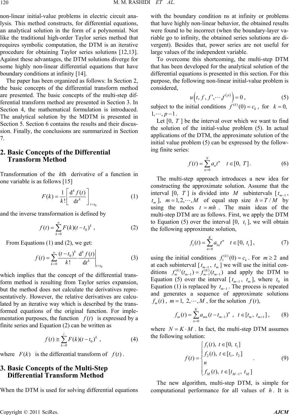

M. M. RASHIDI ET AL. 120
non-linear initial-value problems in electric circuit ana-
lysis. This method constructs, for differential equations,
an analytical solution in the form of a polynomial. Not
like the traditional high-order Taylor series method that
requires symbolic computation, the DTM is an iterative
procedure for obtaining Taylor series solutions [12,13].
Against these advantages, the DTM solutions diverge for
some highly non-linear differential equations that have
boundary conditions at infinity [14].
The paper has been organized as follows: In Section 2,
the basic concepts of the differential transform method
are presented. The basic concepts of the multi-step dif-
ferential transform method are presented in Section 3. In
Section 4, the mathematical formulation is introduced.
The analytical solution by the MDTM is presented in
Section 5. Section 6 contains the results and their discus-
sion. Finally, the conclusions are summarized in Section
7.
2. Basic Concepts of the Differential
Transform Method
Transformation of the thk derivative of a function in
one variable is as follows [15]
0
1d ()
() !d
k
k
tt
ft
Fk kt



(1)
and the inverse transformation is defined by
0
0
()( )()
k
k
f
tFktt



, (2)
From Equations (1) and (2), we get:
0
0
0
() d()
() !d
kk
k
ktt
tt ft
ft kt



 (3)
which implies that the concept of the differential trans-
form method is resulting from Taylor series expansion,
but the method does not calculate the derivatives repre-
sentatively. However, the relative derivatives are calcu-
lated by an iterative way which is described by the trans-
formed equations of the original function. For imple-
mentation purposes, the function ()
f
t is expressed by a
finite series and Equation (2) can be written as
0
0
()( )()
ik
k
f
tFktt


, (4)
where ()
F
k is the differential transform of ()ft.
3. Basic Concepts of the Multi-Step
Differential Transform Method
When the D TM is used f or solving differential equations
with the boundary condition ns at infinity or problems
that have highly non-linear behavior, the obtained results
were found to be in correct (when the boundary-layer va-
riable go to infinity, the obtained series solutions are di-
vergent). Besides that, power series are not useful for
large values of the independent variable.
To overcome this shortcoming, the multi-step DTM
that has been developed for the analytical solution of the
differential equations is presented in this section. For this
purpose, the following non-linear initial-value problem is
considered,



, , ,,0
p
ut fff
, (5)
subject to the initial conditions ()
(0)
kk
f
c, for 0,k

1, ,1p

.
Let [0, T] be the interval over which we want to find
the solution of the initial-value problem (5). In actual
applications of the DTM, the approximate solution of the
initial value problem (5) can be expressed by the follow-
ing finite series:
0
() Nn
n
n
f
tat

 [0, ]tT. (6)
The multi-step approach introduces a new idea for
constructing the approximate solution. Assume that the
interval [0, T] is divided into
M
subintervals [1m t

,
m
t], 1,2,,mM

 of equal step size /hTM by
using the nodes m
tmh

. The main ideas of the
multi-step DTM are as follows. First, we apply the DTM
to Equation (5) over the interval [0, 1 t], we will obtain
the following approximate solution,
11
0
() Kn
n
n
f
tat

 1 [0, ]tt, (7)
using the initial conditions ()
1(0)
kk
f
c. For 2m and
at each subinterval [1m
t

, m t] we will use the initial con-
ditions () ()
111
() ()
kk
mm mm
f
tft

 and apply the DTM to
Equation (5) over the interval [1m
t, m t], where 0 t in
Equation (1) is replaced by 1m
t. The process is repeated
and generates a sequence of approximate solutions
()
m
f
t, 1, 2 ,,mM

, for the solution (),
f
t
1
0
()( )
Kn
mmnm
n
fta tt



, 1
[, ]
mm
ttt

, (8)
where NKM

. In fact, the multi-step DTM assumes
the following solution:
11
212
1
(), [0, ]
(), [, ]
()
(), [, ]
M
MM
ft tt
ft ttt
ft n
f
tt tt









. (9)
The new algorithm, multi-step DTM, is simple for
computational performance for all values of h. It is

M. M. RASHIDI ET AL. 121
Figure 1. Variation fη() with respect to K, when =2M,
1s= , =1a, for the stretching sheet.
Figure 2. Variation  f
η
() with respect to K, when =2M,
1s= , =1a, for the stretching sheet.
easily observed that if the step size ,hT then the
multi-step DTM reduces to the classical DTM. As we
will see in the next section, the main advantage of the
new algo-rithm is that the obtained series solution con-
verges for wide time regions and can approximate
non-chaotic or chaotic solutions.
4. Mathematical Formulation
Consider the flow of a second-order fluid following
Equations (10-12) as
Figure 3. Variation

 f
η
() with respect to K, when
=2M, 1s= , =1a, for the stretching sheet.
Figure 4. Variation f
η
() with respect to M, when
=1K, 1s= , =1a, for the stretching sheet.
2
112 21
AA A,TpI     (10)
where 1
A (gradv)+(gradv)T , and
21 11
A=dA/d +A (gradv)A,
T
t (11)
112
0, 0,0.

  (12)
The flow past a flat sheet coinciding with the plane
0y

, the flow being confined to 0y. Two equal and
opposite forces are applied along the x-axis so that the
wall is stretched, keeping the origin fixed, and a uniform
magnetic field 0
B is imposed along the y-axis. The
steady two-dimensional boundary-layer equations for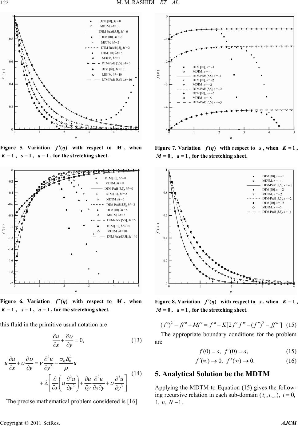

M. M. RASHIDI ET AL. 122
Figure 5. Variation  f
η
() with respect to M, when
=1K, 1s= , =1a, for the stretching sheet.
Figure 6. Variation  f
η
() with respect to M, when
=1K, 1s= , =1a, for the stretching sheet.
this fluid in the primitive usual notation are
0,
u
xy
 

 (13)
2 200
2
223
23
B uu
uu
xyy
uuu u
u
xyxy yy
 
 

 
 



 








(14)
The precise mathematical problem considered is [16]
Figure 7. Variation fη() w ith respect to s, when =1K,
=0 M, =1a, for the stretching sheet.
Figure 8. Variation

f
η
() with respect to s, when =1K,
=0 M, =1a, for the stretching sheet.
22
()[2() ]
i
f
ffMffKf ffff

 
  (15)
The appropriate boundary conditions for the problem
are
(0) , (0),
f
sf a


 (15)
() 0,() 0.ff



 (16)
5. Analytical Solution be the MDTM
Applying the MDTM to Equation (15) gives the follow-
ing recursive relation in each sub-domain (i
t,1i t

), 0,i

1, , 1nN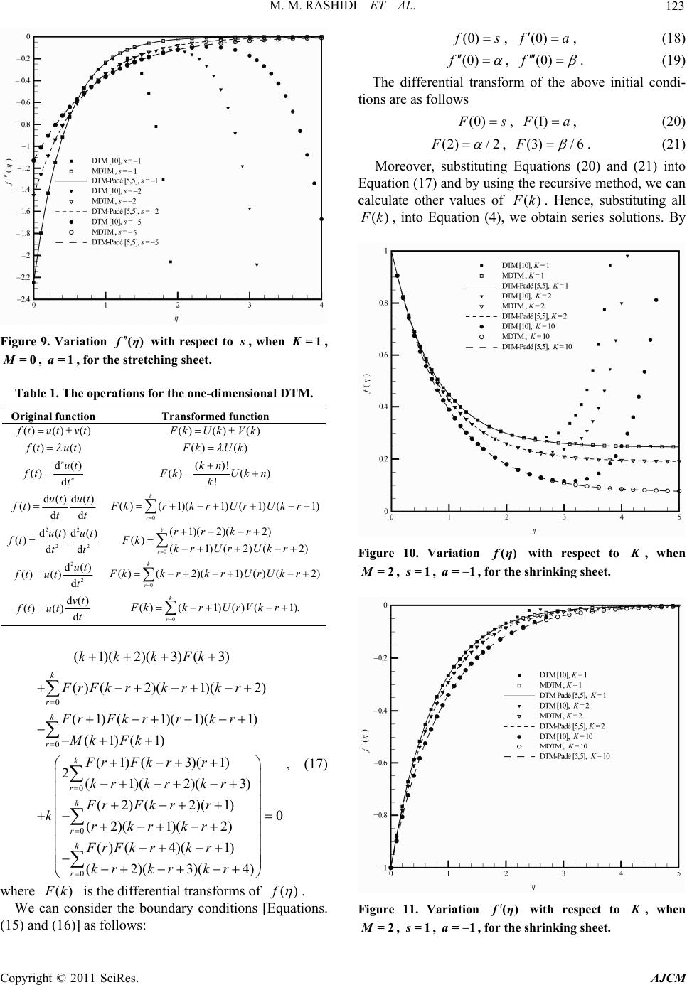

.

M. M. RASHIDI ET AL. 123
Figure 9. Variation  f
η
() with respect to s, when =1K,
=0
M, =1a, for the stretching sheet.
Table 1. The operations for the one-dimensional DTM.
Original function Transformed function
()() ()
f
tutvt ()()()
F
kUkVk
() ()
f
tut

 ()()
F
kUk


d()
() d
n
n
ut
ft t  ()! ()( )
!
kn
F
kUkn
k


d()d()
() dd
ut ut
ft tt  0
()(1)( 1)(1)( 1)
k
r
FkrkrUrUkr

 

22
22
d()d()
() dd
ut ut
ft tt  0
(1)(2)( 2)
() (1)(2)(2)
k
r
rr kr
Fk kr UrUkr

 


 

2
2
d()
()()d
ut
ft utt  0
()(2)(1)()(2)
k
r
Fkkrkr UrUkr



d()
()() d
vt
ft utt  0
()(1)() (1).
k
r
Fkk rUrVk r

 

0
0
0
0
(1)(2)(3)(3)
()(2)(1)(2)
(1)( 1)(1)(1)
(1)(1)
(1)( 3)(1)
2(1)(2)(3)
(2)(2)(1)
(2)( 1)(2)
k
r
k
r
k
r
k
r
kk kFk
FrFkrkrkr
FrFk rrkr
Mk Fk
FrFk rr
kr krkr
FrFk rr
krkrkr




 


 

 

 




0
0
() (4)(1)
(2)(3)(4)
k
r
FrFkrkr
krkrkr









 



 


, (17)
where ()
F
k is the differential transforms of ()f

.
We can consider the boundary conditions [Equations.
(15) and (16)] as follows:
(0)
f
s

, (0)
f
a
, (18)
(0)f




, (0)f

 . (19)
The differential transform of the above initial condi-
tions are as follows
(0)
F
s

, (1)
F
a, (20)
(2)/ 2F


, (3)/ 6F

. (21)
Moreover, substituting Equations (20) and (21) into
Equation (17) and by u sing the recursive method, we can
calculate other values of ()
F
k. Hence, substituting all
()
F
k, into Equation (4), we obtain series solutions. By
Figure 10. Variation f
η
() with respect to K, when
=2M, 1s= ,

=1a, for the shrinking sheet.
Figure 11. Variation

f
η
() with respect to K, when
=2M, 1s= ,

=1a, for the shrinking sheet.

M. M. RASHIDI ET AL. 124
Table 2. Comparison of obtained results for 
f(η), when =2M, 1s= and =1a and various values of parameter K.
()f


1.K 2K


DTM Padé [5, 5] MDTM DTM Padé [5, 5] MDTM
0.0 1.00000 1.00000 1.00000 1.00000 1.00000 1.00000
0.5 0.716312 0.706233 0.706233 0.761281 0.747084 0.747084
1.0 0.558208 0.498765 0.498765 0.643042 0.558134 0.558134
1.5 0.507194 0.352244 0.352244 0.641502 0.416973 0.416973
2.0 0.549619 0.248766 0.248766 0.754462 0.311513 0.311513
2.5 0.671554 0.175687 0.175687 0.975226 0.232727 0.232727
3.0 0.779422 0.124076 0.124076 1.16384 0.173866 0.173866
3.5 0.467092 0.0876271 0.0876264 0.645226 0.129893 0.129893
4.0 –1.51143 0.0618864 0.0618847 –2.73495 0.0970411 0.0970406
4.5 –8.28107 0.0437091 0.043705 –14.5163 0.0724986 0.0724975
5.0 –26.7055 0.0308744 0.0308659 –47.0937 0.0541641 0.0541617
5.5 –70.4832 0.0218145 0.0217985 –125.568 0.0404682 0.0404633
6.0 –165.017 0.0154227 0.0153948 –297.038 0.0302383 0.0302295
6.5 –354.731 0.0109179 0.0108723 –644.682 0.022599 0.0225839
7.0 –713.66 0.00774892 0.00767839 –1308.26 0.0168963 0.0168721
7.5 –1360.3 0.00552703 0.00542273 –2513.06 0.0126421 0.0126049
8.0 –2477.92 0.00397796 0.00382971 –4609.63 0.00947179 0.00941688
8.5 –4341.63 0.0029083 0.00270467 –8127.06 0.00711334 0.0070352
9.0 –7353.9 0.00218163 0.00191012 –13843.1 0.00536369 0.00525588
9.5 –12090.3 0.00170165 0.00134899 –22874.4 0.00407131 0.00392658
10 –19357.2 0.00140031 0.000952703 –36792.3 0.00312311 0.00293349
Table 3. Comparison of obtained results for  f(η), when =2M, 1s= and =1a and various values of parameter K.
()f




1.K 2K


DTM Padé [5, 5] MDTM DTM Padé [5, 5] MDTM
0.0 0.695621 0.695621 0.695621 0.583156 0.583156 0.583156
0.5 0.437262 0.49127 0.49127 0.359195 0.435667 0.435667
1.0 0.202525 0.346951 0.346951 0.116804 0.325479 0.325479
1.5 0.00605472 0.245028 0.245028 –0.109835 0.24316 0.24316
2.0 –0.173392 0.173047 0.173047 –0.343373 0.181661 0.181661
2.5 –0.290258 0.122211 0.122211 –0.505173 0.135716 0.135716
3.0 –0.0223928 0.0863097 0.0863097 –0.0537612 0.101391 0.101391
3.5 1.65387 0.0609548 0.0609548 2.78564 0.0757477 0.0757477
4.0 7.24184 0.0430483 0.0430482 12.4698 0.0565899 0.0565899
4.5 22.024 0.0304023 0.0304021 38.5972 0.0422774 0.0422774
5.0 56.0808 0.0214713 0.0214709 99.7758 0.0315848 0.0315847
5.5 127.258 0.0151642 0.0151635 229.359 0.0235966 0.0235964
6.0 265.338 0.0107103 0.010709 483.575 0.0176288 0.0176285
6.5 517.708 0.00756533 0.00756301 952.633 0.0131705 0.01317
7.0 956.839 0.00534496 0.00534125 1775.47 0.00984004 0.00983907
7.5 1689.93 0.00377781 0.00377216 3158.83 0.00735216 0.0073506
8.0 2871.07 0.00267225 0.00266403 5401.49 0.00549389 0.00549152
8.5 4716.41 0.00189295 0.00188142 8924.45 0.0041061 0.00410262
9.0 7522.61 0.00134434 0.00132872 14308. 0.00306991 0.003065
9.5 11689.3 0.000958921 0.000938387 22336.5 0.00229654 0.00228981
10 17745.6 0.000689019 0.00066272 34052.4 0.00171964 0.00171068
using the asymptotic boundary condition (2)/ 2F


and () 0f , we can obtain

,

. For analytical
solution of the considered problem, the convergence
analysis was performed and in Equation (4), the i value
is selected equal to 10 and the interval was set equal to
0.01.
6. Results and Discussion
Equation (15) with transformed boundary conditions was
solved analytically using the DTM and the MDTM. In
order to give a comprehensive approach of the problem,
a comparison between DTM, MDTM and DTM-Padé
solutions for various param e ters is presente d.
In Figures 1-9, solutions for the stretching sheet are
illustrated. Figures 1-3 show the variation of ()f

,
()f


, ()f


 for various values of
K
. It is observed
that increasing the parameter
K
. causes increases in
()f

, ()f


, profiles, respectively. The influence of
the magnetic parameter
M
, on ()f

, ()f

, ()f




M. M. RASHIDI ET AL. 125
Figure 12. Variation  fη()
with respect to K, when
=2M, 1s= , =1a, for the shrinking sheet.
Figure 13. Variation f
η
() with respect to M, when
=1K, 5s=, =1a, for the shrinking sheet.
is presented in Figures 4-6. It can be concluded that, an
increase in the magnetic parameter decreases ()f

,
()f

, profiles. The effects of the parameter
s
are
shown in Figures 7-9. It is clear that an increase in this
parameter causes a remarkable rise in ()f

profile.
Conversely, an increase in the value of ,s causes a
corresponding decrease in ()f

 profile.
In Figures 10-18, solutions for the shrinking sheet are
shown. Figures 10-12 show the variations of ()f

,
()f

, ()f

 for various values of
K
. It is observed
that increasing the parameter
K
. causes decreases in
()f

, ()f

, profiles, respectively. The influence of
Figure 14. Variation

fη() with respect to M, when
=1K, 5s= ,

=1a, for the shrinking sheet.
Figure 15. Variation


fη() with respect to M, when
=1K, 5s=,

=1a, for the shrinking sheet.
the magnetic parameter
M
, on ()f

, ()f

, ()f



is presented in Figures 13-15. It can be concluded that,
an increase in the magnetic parameter increases ()f

,
In Figures 10-18, solutions for the shrinking sheet are
shown. Figures 10-12 show the variations of ()f

,
()f


, ()f


 for various values of K. It is observed
that increasing the parameter K. causes decreases in
()f

, ()f


, profiles, respectively. The influence of
the magnetic parameter
M
, on ()f

, ()f

, ()f



is presented in Figures 13-15. It can be concluded that,
an increase in the magnetic parameter increases ()f

,
()f


, ()f


 profiles. The effects of the parameter

M. M. RASHIDI ET AL. 126
Figure 16. Variation fη() with respect to s, when =1K,
=2M, =1a, for the shrinking sheet.
Figure 17. Variation  fη()
with respect to s, when
=1K, =2M, =1a, for the shrinking sheet.
,s are shown in Figures 16-18. It is clear that increas-
ing this parameter causes a remarkable rise in ()f

profile. Conversely, increasing the value of
s
,
causes a decrease in ()f

 profile. The Residual
errors for Equation 15 are plotted in Figures 19-20 using
the DTM and MDTM respectively. In order to verify the
efficiency of the proposed method in comparison with
the DTM and DTM-Padé solutions, we report the ob-
tained results in Tables 2 and 3 for ()f

and ()f


when 2
M
, 1s and 1x

and various values of
the parameter
K
. for ()f

 and ()f


, respectively.
It is obvious from Tables 2 and 3 that the MDTM is a
Figure 18. Variation


f
η
() with respect to s, when
=1K, =2M,

=1a, for the shrinking sheet.
Figure 19. Residual error for Equation (15) using the DTM
approximations when =1K, =2M, 5s= and

=1a.
reliable algorithm method.
7. Conclusions
In this paper, the Multi-step differential transform me-
thod was applied successfully to find the analytical solu-
tion of resulting ordinary differential equation for the
problem of flow of a second-grade fluid over a stretching
or shrinking sheet. The present method reduces the
computational difficulties of the other methods (same as
the HAM, VIM, ADM and HPM) [17-19], on the other
hand, this method has some limitations (respect to HAM,

M. M. RASHIDI ET AL. 127
Figure 20. Residual error for Equation (15) using the
MDTM approximations when =1K, =2M, 5s= and
=1a.
VIM, ADM and HPM). The method has been applied
directly without requiring linearization, discretization, or
perturbation. The accuracy of the method is excellent.
The obtained results demonstrate the reliability of the
algorithm and give it a wider applicability to non-linear
differential equations.
8. References
[1] S. K. Ghosh, O. A. Bég, R. Bhargava, S. Rawat and T. A.
Bég, “Mathematical Modelling of Transient Magnetohy-
drodynamic Couple Stress Biofluid Flow in a Rotating
Channel,” International Journal of Applied Mathematics
and Mechanics, Vol. 6, No. 6, 2010, pp. 23-45.
[2] O. Anwar Bég, H. S. Takhar, R. Bharagava, S. Rawat and
V. R. Prasad, “Numerical Study of Heat Transfer of a
Third Grade Viscoelastic Fluid in Non-Darcian Porous
Media with Thermophysical Effects,” Physica Scripta,
2008, Vol. 77, No. , pp. 1-11.
[3] D. A. S. Rees and A. P. Bassom, “Boundary Layer Flow
of a Micropolar Fluid,” International Journal of Engi-
neering Science, Vol. 34, No. 1, 1996, pp. 113-124.
doi:10.1016/0020-7225(95)00058-5
[4] O. A. Bég, A. Y. Bakier and V. R. Prasad, “Numerical
Study of Free Convection Magnetohydrodynamic Heat
and Mass Transfer from a Stretching Surface to a Satu-
rated Porous Medium with Soret and Dufour Effects,”
Computational Materials Science, Vol. 46, No. 1, 2009,
pp. 57-65. doi:10.1016/j.commatsci.2009.02.004
[5] S. K. Ghosh, O. Anwar Bég and M. Narahari, “Hall Ef-
fects on MHD Flow in a Rotating System with Heat
Transfer Characteristics,” Meccanica, Vol. 44, No. 6,
2009, pp. 741-765. doi:10.1007/s11012-009-9210-6
[6] C. Truesdell and W. Noll, “The Non-Linear Field Theo-
ries of Mechanics,” In: S. Flügge, Ed., Encyclopedia of
Physics, III/3, Springer, Berlin, 1965, pp. 1-591.
[7] K. R. Rajagopal, “On Boundary Conditions for Fluids of
the Differential Type,” In: A. Sequeira, Ed., Navier-
Stokes Equations and Related Non-linear Problems, Ple-
num Press, New York, 1995, pp. 273-278.
[8] K. R. Rajagopal and P. N. Kaloni, “Some Remarks on
Boundary Conditions for Fluids of the Differential Type,”
In: G.A.C. Graham and S. K. Malik, Eds., Continuum
Mechanics and Its Applications, Hemisphere, New York,
1989, pp. 935-942.
[9] K. R. Rajagopal and A. S. Gupta, “An Exact Solution for
The Flow of a Non-Newtonian Fluid Past an Infinite
Plate,” Meccanica, Vol. 19, No. 2, 1984, pp. 158-160.
doi:10.1007/BF01560464
[10] Z. M. Odibat, C. Bertelle, M. A. Aziz-Alaoui, G. H. E.
Duchamp, “A Multi-Step Differential Transform Method
and Application to Non-Chaotic or Chaotic Systems,”
Computers and Mathematics with Applications, Vol. 59,
No. 4, 2010, pp. 1462-1472.
doi:10.1016/j.camwa.2009.11.005
[11] J. K. Zhou, “Differential Transformation and Its Applica-
tions for Electrical Circuits,” Huazhong University of
Science and Technology Press, Wuhan, 1986, (in Chi-
nese).
[12] M. M. Rashidi and M. Keimanesh, “Using Differential
Transform Method and the Padé Approximant for Solv-
ing MHD Flow in a Laminar Liquid Film from a Hori-
zontal Stretching Surface,” Mathematical Problem in En-
gineering, Vol. 2010, Article ID 491319.
[13] M. M. Rashidi, M. Keimanesh, O. Anwar Bég and T. K.
Hung, “Magnetohydrodynamic BioRheological Transport
Phenomena in a Porous Medium: A Simulation of Mag-
netic Blood Flow Control and Filtration,” International
Journal for Numerical Methods in Biomedical Engineer-
ing, Vol. 27, No. 6, 2011, pp. 805-821.
doi:10.1002/cnm.1420
[14] M. M. Rashidi, “The Modified Differential Transform
Method for Solving MHD Boundary-Layer Equations,”
Computer Physics Communications, Vol. 180, No. 11,
2009, pp. 2210-2217. doi:10.1016/j.cpc.2009.06.029
[15] I. H. Abdel-Halim Hassan, “Comparison differential
Transformation Technique with Adomian Decomposition
Method for Linear and Nonlinear Initial Value Prob-
lems,” Chaos Solitons and Fractals, Vol. 36, No. 1, 2008,
pp. 53-65. doi:10.1016/j.chaos.2006.06.040
[16] A. Robert Van Gorder, “High-order Nonlinear Boundary
Value Problems Admitting Multiple Exact Solutions with
Application to The Fluid Flow over a Sheet,” Applied
Mathematics and Computation, Vol. 216, No. 7, 2010, pp.
2177-2182. doi:10.1016/j.amc.2010.03.053
[17] M. M. Rashidi and H. Shahmohamadi, “Analytical Solu-
tion Of Three-Dimensional Navier-Stokes Equations for
the Flow Near an Infinite Rotating Disk,” Communica-
tions in Nonlinear Science and Numerical Simulation,
Vol. 14, No. 7, 2009, pp. 2999-3006.
doi:10.1016/j.cnsns.2008.10.030

M. M. RASHIDI ET AL. 128
[18] M. M. Rashidi and S. Dinarvand, “Purely Analytic Ap-
proximate Solutions for Steady Three-Dimensional Prob-
lem of Condensation Film on Inclined Rotating Disk by
Homotopy Analysis Method,” Nonlinear Analysis: Real
World Applications, Vol. 10, No. 4, 2009, pp. 2346-2356.
doi:10.1016/j.nonrwa.2008.04.018
[19] M. M. Rashidi, S. A. Mohimanian pour and S. Abbas-
bandy, “Analytic Approximate Solutions for Heat Trans-
fer of a Micropolar Fluid Through a Porous Medium with
Radiation,” Communications in Nonlinear Science and
Numerical Simulation, Vol. 16, No. 4, 2011, pp.
1874-1889
Nomenclature
0
B uniform magnetic field along the y-axis
M
magnetic parameter
R suction parameter

viscoelastic parameter

kinematic viscosity
0

electric conductivity