American Journal of Computational Mathematics, 2011, 1, 39-54
doi:10.4236/ajcm.2011.12005 Published Online June 2011 (http://www.scirp.org/journal/ajcm)
39
Characteristic Analysis of Exponential Compact Higher
Order Schemes for Convection-Diffusion Equations
Sanyasiraju V. S. S. Yedida, Nachiketa Mishra
Department of Mathematics, Indian Institute of Technology Madras, Chennai, India
Received February 19, 201 1; revised March 23, 20 1 1; accepted April 5, 2011
Abstract
This paper looks at the development of a class of Exponential Compact Higher Order (ECHO) schemes and
attempts to comprehend their behaviour by introducing different combinations of discrete source function
and its derivatives. The characteristic analysis is performed for one-dimensional schemes to understand the
efficiency of the scheme and a similar analysis has been introduced for higher dimensional schemes. Finally,
the developed schemes are used to solve several example problems and compared the error norms and rates
of convergence.
Keywords: Exponential Scheme, Compact Higher Order Scheme, Characteristics, Resolving Efficiency,
Finite Difference
1. Introduction
Many interesting engineering problems involve the
physical processes and transport phenomena that include
fluid flow, heat and mass transfer, can be modelled by a
general Convection-Diffusion Equation (CDE). This
equation describes the convection and diffusion chara-
cteristics of various physical quantities, such as mome-
ntum, energy, concentration, etc. This paper deals with
the numerical solution of convection-diffusion equation
of the form
=(, )
xxyy xy
aubucuduf x y  (1)
on , with boundary conditions
2
R
(, )=(, )ux ygx y on  , (2)
where are constant diffusion, , are
constant convection coefficients and
, >0ab cd
f
,
g
are
sufficiently smoo th functions with resp ect to
x
and .
If , are very small when compared with
and , then (1) becomes a convection dominated
equation for which [1-4] are some of the exponential
schemes known from the literature. For higher dim-
ensional problems, though the schemes [2-4] are all
fourth order accurate, scheme presented in [4] seems to
be giving better results over the other two. The purpose
of this work is to understand the good features of the
scheme given in [4] and based on these features include
some additional condition s in the development of ECHO
schemes. Since the development of these schemes is
already been discussed in [4], instead of repeating the
same in this work, we focus on understanding the merits
of the scheme. Section two presents a new class of
ECHO schemes for 1D CDE, their classification and
numerical verification. Echo schemes for 2D CDE are
formulated and compared in the Section three and
conclusions are drawn in the last section.
y
0< a<<1b
d c
2. 1D Convection-Diffusion Equations
The one dimensional e q ui val ent of (1), by fixi ng
, is given by ==0bd
=()
xx x
aucuf x

, , (3) 0< <1x
with boundary conditions , , where
1
(0) =ug 2 (1) =ug
1
g
, 2
g
are some constants.
2.1. ECHO Schemes
A general strategy to develop ECHO schemes is by
starting with the difference equation
2=
hihii
Du cDuF   (4)
where 11 =( )/2
hi ii
Du uuh


and 21 =( 2
hi ii
Du uu



over a uniformly distributed nodal points with
step length and
2
h
hi
1)/ i
u

F
is a linear combination of the
source term i
f
and its derivatives at a chosen number

40 S.V.S.S. YEDIDA ET AL.
of stencil (mesh) points with equal number of arbitrary
constants (refer [2-4] for three such different choices).

is taken to be coth
22
ch ch
a





when the convection
coefficient so that the difference Equation (4) is
exact for
0c
cx
a
e



otherwise it is equal to . If ai
F
is
taken as i
f
then (4) is a second order compact
exponential scheme which was discussed in [5]. In the
development of the ECHO scheme, the arbitrary
constants in i
F
are obtained by making the difference
Equation (4) is exact for
x
, 2
x
, In this work
four different stencils are used for
3,x
i
F
and the
corresponding constants have been computed by forcing
the difference scheme (4) to be at least fourth order
accurate. The four chosen stencils and their constants are
given by (refer [3,4] for the complete derivation of the
computation of the coefficients).
2.1.1. Stencil-1
Consider the discrete source function
11ii23i1 4
=(
i) ix
F
cfc f

cfc f

 (5)
where i
f
, ()
x
i
f
are the source function and it’s
derivative, respectively, at the nodal point . The
i
Equation (4) is already exact for 1, e


23
cx
a








4
,
and
enforcing the exactness also for

, ,
x
xx
4
x gives
four simultaneous equations in terms of its coefficients.
Solving them for , gives
i
c=1 ,i, 2 3 &
32
1=0.25c2
1
630.5 3
 
 ,
2
22
=2 2
3
c

 ,
32 2
3=0.25c1
630.5 3
  

0.5

32
6


 ,
4
ch=6

 , =a
ch
 , =ch


for 0c

and 11
=12 c, 25 =6 c, 31
12
13
c
=

c c
)

, when .
4=0c=0
1
Similarly for the other stencils, system of equations
are obtained and solved to get the corresponding co-
efficients.
2.1.2. Stencil-2
12
=()()(
i ixixi
fcffc

0
4xi
fFc (6)
when the coefficients are c
1=1c,
32
11
.5
61
2
21
=0 0.5
212
ch





 


,
32
325
=2 2
36
ch






,
32 2
4111
=0.50
61212
ch .5

 





and ,
1=1c2=24
h
c

, ,
3=0c4=24
h
c for c. =0
)
2.1.3. Ste n ci l-3
12 34
=()()(
iixixx ixxxi
Fcfcf cfcf

 , (7)
when 0c

the coefficients are
1=1c, 2=( )ch



, 22
31
=6 ch






,
33
4=ch 2
11
612

 

 


,
and , ,
1=1c2=0c
2
3=12
h
c, for .
4=0c=0c
()
i
2.1.4. Ste nc i l - 4
11 231 45
=()
iiiixixx
F
cfc fcfcfcf


  (8)
when 0c

the coefficients are
43 2
1=123(14)(23 )
(0.5)(0.10.25)
c
 
 

 ,
432
2=24 244 20.8c
  
43 2
3=123(14 )(23 )
(0.5)(0.10.25)
c
,
 


,
32
4=(660.5ch )

   ,
24 32
1
=1212 15 ch
 

5



,
and 11
=30 c, 214 =15 c, 31 =30 c, ,
4=0c
2
5=20
h
c
for .
=0c
Schemes with stencils 1, 2 and 3 contain four
parameters and are fourth order accurate, whereas the
scheme with stencil 4 contains five parameters and is
sixth order accurate. Here after, we refer the difference
scheme (4) with stencils 1 to 4 as schemes [1 ]
1
D
S to
[1 ]
4
D
S, respectively for all the future references.
Exponential schemes of [2,3] are also fourth order
accurate with three arbitrary parameters and the scheme
given in [4] uses six parameters to generate a sixth order
scheme for the chosen one-dimensional convection-

S.V.S.S. YEDIDA ET AL.
41
diffusion equation. The discrete source terms of these
schemes [2-4] ar e gi v en by.
Stencil used in [2]:
11
=
ii2 31ii
F
cfc fc f

 (9)
2
11
=0.50.5
6
c

  , 2
22
=2 2
3
c

 ,
2
31
=0.50
6
c.5

  when 0c

,
11
=12 c, 25
=6 c, 31
=12 c when =0c.
Stencil used in [3]:
)
i12
=3 ()(
iixixx
F
cfcfc f (10)
c, ch
1=1 2=( )

 , 22
31
=6 ch






when ,
0c
1=1c, 2=0c, 2 3=12
h
c when =0c.
Stencil used in [4]:
1
11
=2 31
4156
()()()
ii ii
x
ixix
cfcf
cfcf cf




i
(11)
when the coefficients are
Fcf
0c
54
90(1290)3
1=(7.512 )
7
(0.5)0.375
30
c

   
 

 ,
43
28
=2424 2
15
c

 ,
54 3
3=90(1290 )(7.512 )
7
(0.5)0.375
30
c

 
 
 
 ,
54 3
42
306(15 )(3.56 )
=1
(0.5 )5
30
ch

 
 





 




5432
5= (12012082)ch

,

  ,
54 3
62
306(15 )(3.56 )
=1
(0.5 )5
30
ch

 











,
and 12 =15 c, 211 =15 c, 32 =15 c, 4=40
h
c, 5=0c,
6=40
h
c for =0c.
Name the scheme (4) with stencils used in [2-4] as
schemes [1 ]
5
D
S, [1 ]
6
D
S and [1]
7
D
S, respectively. That is,
a total ofn O sche have been introduced
until now and out of which five of them are fourth order
accurate and the other two are sixth order accurate.
Among the fourth order schemes, three of them,
developed in this work, have four free parameters and
the other two, taken from the literature [2] and [3], have
three parameters. Among the sixth order schemes, one
scheme developed in this work has five free parameters
and the other taken from the literature [1]
7
seveECHmes
D
S has six
parameters. That is, the seven schemes canlassified
into th
n order schemes with n number of parameters
and tther contain less than number of parameters.
The aim of the rest of the works to demonstrate, using
wave number analysis and numerical experimentation,
the th
n order ECHO schemes with n parameters are
more accurate than the other class of scmes.
be c
ution
he o
2.2. Com
g th
n
i
arison of the Characteristic Curves
alys
he
, re
p
Usie wave number anissolof any n
numerical scheme can be measured with which one can
understand the closeness of the characteristic of a
difference equation to that of the differential equ ation [6].
Since the stability of any numerical scheme depends on
the magnitude of the peclet number, defined by =ch p,
in this work, the characteristics are comparh
respect to peclet numbers. The characteristic of the
governing Equation (1), obtained by sub stituting
a
ed wit
I
wx
e in
the place of the dependent variable u, is given by:
2
c
[1 ]= D
I
hp




 (12)
wh

ere =wh

, is the nuwe wavmber, =1I

.
schemeSimilarha teristics of the differences
are obtained by substituting
ly, the crac
I
i
e

at i u to get (refer
[4,6] for more details).
Characteristic Cur[1D]
1
S
ve for :
''
2



'
1
z

[1 ]
1=
D
hzI

 (13)
wh
cwIw


ere w'=sin

, ''=2 2wcos

, 1 =coth
22
p



, 
14 31
=()sinz

 

, 231 )co=( sz

 , 
32
13
=p
11
0.250.5)) 3
6
ppp  


((3 1 


 


,
2
22
12
=2  2 ,
3pp p



32
33
=p
11
0.251 3
6
ppp  (3)( 0.5)




 
 


, 

42 S.V.S.S. YEDIDA ET AL.
3
43
1
= (0.566)pp
p




teristic Curve for [1D]
2
.
Charac
S
:
'' '
[1 ]
2=
D
hz


 21
cwIw
zI


 

(14)
where
 sin=
'
w, ''=2 2cosw

,
1
 )cosz=c
oth
22
p



,1342 =(

 
2
)sin
  ,
21
=(z4

 , 1=1

,
32
231)1pp
p

 



,
111
=0
.5(
12 6p





 ()
2
152
=2(
63
pp 



 


,
331)
p
32
43
111
=0.5(1)
12 6
pp p
p




 


.
Characteristic Curve for
(1  )
[1D]
3
S
:
'' '
21
cwIw
I


 (15)
where
[1 ]
3=
D
hz z



'=sinw

, ''=2 2cosw

, 1
=coth
22
p




,
2
4
)
12
=(z

 , 21 =z2
3

 , 1=1

,
21
=(1 )p
p

 , 2
32
11
=1
6pp p






,
23
43
=1
p
111
61
pp p
2








.

Characteristic Curve for [1D]
4
S
:
''

'
21
cwIw

 (16)
where θ(λ) [2]S4
[1 ]
4=
D
hz Iz



'=sinw

, ''=2 2cosw

, 1 =coth
22
p




,
14 1
)
3
=(zsin

 
2
225
=(
  ,
31
)
[1D]
λ
Figure 1. Comparison of real and imaginary parts of
at =0.1p.
23 4
24
1
={2424420.8}ppp p
p
  ,
2
cosz

     , 
2
1) (
1 0.25
pp
1
p4
34
=( 123(14
(0.5 )(0.pp
23
))
)








,
34
34
1
=(123(14)(23)
(0.5)(0.10.25))
pp
p
pp






,
3
43
1
=(66 0.5pp
p)


 ,
24
54
11
=121215 pp p
p





.
Both real and imaginary parts of theharacteristics
(13-16) are compared with (12) in Figures, 2 and 3 for
peclet numbers 0.1, 10 and 100, respectively. For the
sake of comparison, the characteristics of t Schemes
c
1
he
[1 ]
5
D
S, [1 ]
6
D
S and [1]
7
D
S, are also included in these
figures. It is clear from these comparisons that the
Scheme [1 ]
7
D
S is the best among the chosen schemes
followed by 1
4
D
S. These comparisons can be quantified
by introducing Resolving efficiency.
2.3. Resolving Efficiency
The resolvingficiency [7] of any numerical scheme, ef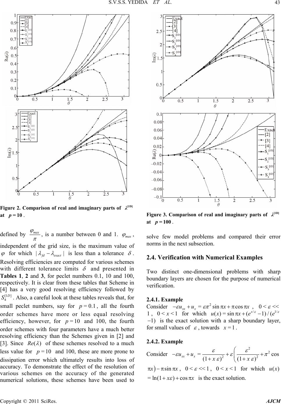

S.V.S.S. YEDIDA ET AL.
43
Figure 2. Comparison of real and imaginary parts of
defined by
[1D]
λ
at =10p.
max


, is a number between 0 and 1. max

,
e ofindependent of the grid size, is the maximum valu

fohicr wh ||
f
d exact

 
Figure 3. Comparison of real and imaginary parts of
at
solve few model problems and compared their error
norms in the next subsection.
Two distinct one-dimensional problems with sharp
Consider x
[1D]
λ
= 100p.
2.4. Verification with Numerical Examples
is less than a tolerance

.
hemesResolving efficiencies aremputed for various sc co
olerance limwith different tits

and presented
Tables 1, 2 and3, for peclet numbers 0.1, 10 and,
respectively. It is clear from these tables that Scheme in
[] has a veryving efficiency followed by
[1 ]
4
in
100
good resol4
D
S. Also, a careful look at these tables reveals that, for
small peclet numbers, say for 0.1p, all the fourth
order schemes have more or less equal resolving
efficiency, however, for =10p and 100, the fourth
order schemes with four parameters have a much better
ving efficiency than the Schemes given in [2] and
[3]. Since ()Re
=
resol

of these schemlved to a much
less value for =10p and 100, these are more prone to
dissipation error which ulty results into loss of
accuracy. To demonstrate the effect of the resolution of
various schemes on the accuracy of the generated
numerical sns, these schemes have been used to
es reso
boundary layers are chosen for the purpose of numerical
verification.
2.4.1. Example 2
=sin cos
xx x
uu x 

0< <<,

1, 0< <1x for which /1/ ()=sin (1)/(
x
uxx ee


 
1)

is the exact solution with a sharp boundary layer,
for small values of

, towards =1x.
2.4.2. Example
imatel
olutio
Csider on22
22
=
(1 )(1 )
xx x
uu xx 




sin
cos



 

x
x

 , 0< <<1

, 0< fo<1xr which ()ux
=ln(1) cos
x
x


 is the exn. act solutio

S.V.S.S. YEDIDA ET AL.
44
Table 1. Resolving efficiency of the real and imaginary
[1D] at =0.1p.
parts of λ
[1 ]
Im( )
D

[1 ]
Re( )
D

Scheme =0.1
 =0  .01 = 0.001  =0.1  =0  .01 = 0.001

[1 ]
1
D
S 0.68 0.39 0.22 0.65 0.38 0.22
[1 ]
2
D
S 0.55 0.30 0.17 0.53 0.30 0.17
[1 ]
3
D
S 70 0.0.0.42 24 0.68 0.42 0.24
[1 ]
4
D
S 1.00 0.75 0.52 0.83 0.60 0.42
Scheme 0.69 0.38 0.21 0.52 0.29 0.16
Schem
[3]
Schem
[4]
[2] e0.70 0.42 0.24 0.55 0.32 0.18
e0.95 0.67 0.45 0.89 0.64 0.44
Table . Ringcien thl ma
pλt p.
2esolv efficy ofe reaand iginary
arts of [1D] a=10
[1 ] e( D  R) [1 ] (D  Im)
Scheme =0.1
 =0.01  = 0.001  =0.1  =0.01  =0.001 
[1 ]
1
D
S 0.59 0.32 0.18 0.68 0.37 0.21
[1 ]
2
D
S 0.44 0.24 0.13 0.52 0.28 0.16
[1 ]
3
D
S 56
[1 ]
0.0.33 0.19 0.63 0.37 0.22
4
D
S
Sch
0.64 0.36 0.20 0.95 0.66 0.45
e 0.16 0.05 0.01 0.77 0.39 0.20
Schem
[3]
Schem
[4]
em
[2] e 0.18 0.05 0.01 0.63 0.42 0.24
e 0.87 0.59 0.45 1.00 0.69 0.46
Table3. lviffic of r
ga λt 0p.
Resong eiency theeal and ima-
inary prts of[1D] a=10
[1 ]
e( D  R) [1 ] (D  Im)
Scheme =0.1

=0.01

=0.001

=0.1

=0.01

=0.001

[1 ]
1
D
S 0.31 0.16 0.11 0.74 0.42 0.21
[1 ]
2
D
S 0.21 0.16 0.11 0.53 0.32 0.16
[1 ]
3
D
S 0.26 0.63 0.37 0.21
[1 ]
0.16 0.11
4
D
S
Sch e
0.36 0.21 0.16 0.89 0.63 0.42
0.05 0.05 0.05 0.58 0.32 0.21
Schem
[3]
Schem
[4]
em
[2] e0.05 0.05 0.05 0.52 0.32 0.21
e0.57 0.42 0.26 1.00 0.73 0.52
Mol .1.) (2.edg
tn es
deproblems (2.4 and4.2.) are solv usin
he seveschem [1
1]
D
S and [1
7]
D
S. To heet
nthmber desriomto
81 theusiramhasn v bn
1 Thorsputy
or pared in the Tables 4 and 5 for problems
1.2
of the error
vary t pecl
umber,
ande nu diffof on pa
no has bee
eter n va beeed fr aried 11 etwee
0–1 and
m, are com
10–4. e err, comted using the infini
n
(2.4.1.) and (2.4.2.), respectively (read 1.234567(–08) as
34567×10 –08 in all these tables).
The comparison norms for various
schemes reveals that for the peclet number p less than
one, the accuracy of all the fourth order schemes are
more or less equal however, the accuracy of the solutions
of the 1
1
D
S to 1
3
D
S becomes better over schemes in [2]
and [3] if p is increased to 1. The improvement in the
accuracy becomes even better, better bydecimal
pl two
o
aces, if p is increased to 10 or more. This behavior
supports the characteristic analysis carriedut in the
earlier section wherein we have shown that the resolving
efficiency of schemes in [2] and [3] is much smaller than
the othurther schemes at large peclet numbers.
This concles that to develop fourth order schemes
using four parameters may improve the resolving
efficiency nd hence the accuracy of the numerical
schemes. The same is also can be concluded between the
sixth order schemes. The solutions generated using
Scheme in [4] are uniformly far superior, for the entire
range of peclet numbers 0.1 to 100, over all the schemes,
wher e as 1
4
er fo
u
a
ord
d
D
S is comparable only at low peclet numbers.
Further, between the three developed fourth order
schemes, 1
2
D
S has less resolving efficiency and the
solutions obtained using this scheme are slightly inferior
when compared with the other two, however, it is still
has a better performance than the two existing three
parameter schemes.
3. 2D Convection-Diffusion Equations
Efficiency of every numerical scheme can be established
computationally by solving a class of example problems
but analysis of the used numerical scheme is more
important to gain confidence before applying them for
real world problems. Usually, the efficiency of the higher
ionary
city or
order compact schemes for one-dimensional stat
CDE is shown by studying their monotoni
comparing their characteristic curves. For 2D schemes,
the comparisons have to be made characteristic surfaces.
The development of a 2D scheme for the two-
dimensional CDE (1) is already presented in [4] and
using a similar procedure, 2D equivalents for the
schemes 1
1
D
S to 1
4
D
S can be developed as follows:
3.1. ECHO Schemes
The development of an ECHO scheme for a two
dimensional CDE will be given in a general procedure
such that a similar procedure can be followed for
different urce nctions. When the convection
coefficients ae constant, the two-dimensional equivalent
so fu
r
*
(17)
of (4) is given by
22
,,,,,
where 1, 1,
=( )/2
hiji ji j
Du uuh

=
hhijkkijh ijkijij
DuDucDu dDuF   

, 21, =( 2
hijijij
Du uu


S.V.S.S. YEDIDA ET AL.
45
orr the example 2.4.1. Table 4. Comparison of the err norms fo

N
p
Scheme [4] S cheme [3][1 ]
4
D
S [1 ]
3
D
S [1 ]
2
D
S [1]
1
D
S
Scheme [2]
11 1
9.09604(–08)2.49708(–04) 3.72418(–04)5.82331(–07)2.77555(–05) 1.08028(–04) 4.03898(–05)
1
10 21 1/2 06) 6.76222(–06) 2.53384(–06)
41 107) 4.22750(–07) 1.58500(–07)
81 1/86 9 2.22867(2)6.60876(9) 2.64234(8) 9.90844()
8
1
3.5212 (–13)8.1183(–07)1.2121(–06)2.8979(–11) 6.8925(–09) 2.6886(–08) 1.0002(–08)
1
8
1
3.7719 (–13)3.7565(–06)4.7198(–06)1.1770(–10) 1.3772(–08) 3.8337(–08) 1.2307(–08)
1
8 1
3.8169 (–13)4.8880(–06)5.0416(–06)1.2949(–10) 1.8805(–08) 4.4755(–08) 1.3008(–08)
1.43583(–09)1.77531(–05)2.33358(–05)9.10599(–09) 1.70241(–
/4
2.24904(–11)9.74330(–07)1.46099(–06) 1.42770(–10)1.05873(–
3.51524(–13) .09526(–08) .14209(–08) –1–0–0–09
11 10
8.88729(–08)1.77531(–03)2.29850(–03) 3.65241(–06)4.88874(–05) 1.37564(–04) 4.53176(–05)
2
10 21 5 1.44506(–09)1.62385(–04)2.29640(–04) 8.90909(–08) 2.43375(–06) 7.90343(–06) 2.75463(–06)
41 2.5
2.25920(–11)1.22054(–05)1.79906(–05) 1.72607(–09)1.22122(–07) 4.48986(–07) 1.63784(–07)
1.25107970 4
11 008.77791(–08) 2.45467(–03) 2.54243(–03) 4.19056(–06) 6.92138(–05) 1.61527(–04) 4.75106(–05)
3
10 21 50
1.48553(–09)2.97753(–04)3.20284(–04) 1.31316(–07) 4.37339(–06) 1.06444(–05) 3.17153(–06)
41 25
2.40075(–11)3.46001(–05)3.96217(–05) 4.02580(–09)2.56511(–07) 6.58354(–07) 2.01890(–07)
12.5738654 7
11 0008.74623(–08) 2.54393(–03)2.54569(–03) 4.20028(–06) 7.21326(–05) 1.64144(–04) 4.74090(–05)
4
10 21 500
1.48149(–09)3.19490(–04)3.21770(–04) 1.32418(–07)4.75839(–06) 1.10378(–05) 3.17837(–06)
41 250
2.40094(–11)3.97058(–05)4.03276(–05) 4.14605(–09)3.02745(–07) 7.10714(–07) 2.05097(–07)
1 25 931609 3
T 5.able Comparison of the error norm for the example 2.4.2.

N
p
Scheme [4] Scheme [3]Scheme [2][1 ]
4
D
S [1 ]
3
D
S [1 ]
2
D
S [1 ]
1
D
S
11 1
1.43890(07)1.94626(04)2.89270(04)4.22688(07)4.32687( 05) 1.70161(04) 6.35454(05) – – – – – – –
1
10 21 ) 1.04996(–05) 3.93304(–06)
41 1/4
3.49160(–11) 7.83288(–07) 1.17424(–06) 1.06559(–10) 1.64206(–07) 6.56127(–07) 2.45980(–07)
81 1/8547) 1.67111(11) 1.02436(8) 4.09636(8) 1.53605()
8 1
6.9841 (13)4.1643 (07)6.2148 (07)1.4773 (11)1.3648 (08) 5.3307(08) 1.9829(08 )
100
1/2
2.23695(–09) 1.24756(–05) 1.86690(–05) 6.76779(–09) 2.63582(–06
.45044(–13).90114(–08).35061(–08 – –0–0–08
11 10
1.96384(–07)8.40121(–04) 1.06619(–03) 1.67762(–06) 1.04588(–04) 3.00805(–04) 9.83965(–05)
2
10 21 5 2.97619(–09)8.06763(–05) 1.13353(–04) 4.36902(–08) 4.94140(–06) 1.62042(–05) 5.63472(–06)
41 2.5
4.51730(–11)
–
6.21577(–06)
–
9.14492(–06)
–
8.72299(–10)
–
2.42789(–07)
–
8.96202(–07)
–
3.26724(–07)
–
1.25 7690931
11
2.00935(–07)1.12598(–03) 1.13629(–03) 1.85818(–06) 1.52895(–04) 3.65401(–04) 1.06674(–04)
3
10 21 50
3.16771(–09)
4.94835(–11)
1.42618(–04)
1.69497(–05)
1.51699(–04)
1.93126(–05)
6.19806(–08)
1.95897(–09)
9.18371(–06) 2.2584
5.25029(–07)
0(–05) 6.7064
1.35391(–06)
9(–06)
4.14529(–07)
41 25
81
12.5
7.64628(–13)1.86159(–06) 2.33386(–06) 5.81487(–11) 2.78268(–08) 7.76336(–08) 2.49046(–08)
11 1000
2.00962(–07)1.16355(–03) 1.13359(–03) 1.85569(–06) 1.59831(–04) 3.72624(–04) 1.06834(–04)
4
10 21 500
3.16938(–09)1.52631(–04) 1.51914(–04) 6.23029(–08) 1.00195(–05) 2.34902(–05) 6.74224(–06)
41 250
4.96365(–11)1.94022(–05) 1.95976(–05) 2.01159(–09) 6.21278(–07) 1.46575(–06) 4.22341(–07)
81 125
7.76046(–13)2.41622(–06) 2.48556(–06) 6.37930(–11) 3.80936(–08) 9.08791(–08) 2.63944(–08)
and
2
1, ) ij
uh


,1 ij ij
uu

nodal poin
2=(
kij
Du / D,1ij,1 )/2
ijk , =( kij
u uu
2
k

ove uniforml
step lengths h and k
,
2)
ij
u
ts with
1/ r ay di
alstributed ong
x

and y

directions, respectively and discrete source
function ij
F
is a 2D
developm
e
e
quivalent of
ent of th the corresp 2D ECHOonding 1D scheme isscheme. The

46
given ellow for erent seon
3.1.1. Schem
S.V.S.S. YEDIDA ET AL.
bdifflectiof source functions.
e [1
1D]
S
urce Consider the sofu
(18)puted using Taylor series
,
nction, which is an extension of
the scheme 2.1.1., given by
*11,2 31,4
1,1 23,1 4
=()
()
ijijijx i
ijijijy ij
Fcf cfcfcf
dfdfdfdf


 
 (18)
The truncation error of the scheme (17) with the
ij
source function com
expansion, is g iy, ven b
,
=,
4
,,
()
x
yij
TE EuGuHu
xyyij xxyij
xxyyi ji j
Ku fOh (19)
where ,
11
=EdKcL, 12 =GbKcL 21 =
H
dK aL

,
22
=
K
bK aL
2
13142 31
131
=(), =()/2,
=( )
Khcc cK hcc
Lkdd
 
 (20)
2
42 31
, =()/2dL kdd
Expanding the terms in (19) and (20) sh
scheme (17) is of second order accurate.
fourth order, the scheme and the source function is
as
e coefficients and ,
are given by
ows that the
To make it
written
2


2
2222
=
hh kkhkhk
khh kh kijij
DDcDdDEDD
GD DHD DKD DuF
  
  (21)
,11,2,31,4,
1,12,3,1 4,
=
ijijiji jxij
ijijijyij
Fcf cfcf cf
dfdf dfdf




where th i ci d=1, 2, 3&4i
32 2
11
= 30.530.25
6
x
xxxxxx
cx

,
2
22
=2 2
3
x
xx
c

 ,
32 2
3=30.5 3
6
10.25
x
xxx
cxxxx
 
,
32 2
11
= 30.530.25
6
y
yyyyyyy
d

 ,
2
22
=2 2
3
y
yy
d

 ,
32 2
31
= 30.530.25
6
y
yyyyyy
dy
 
,
32
4=(60.5 6)
y
yyy
dh

 ,
=
x
a
ch
 , =
y
a
dk
 , =h
xch

 , and =k
ydk


for and not equal to zero cd
and 11, =c12 25, =c631 =c12, =0c4, 11 =d12 ,
25
=6 d, 31 =12 d, 4=0d when.
Similarly, for the other selection of source functions
remainder terms are utilized to get fourth order accuracy.
For every sche
0==cd
me , E, G
H
K
aras i and e same n
(20) but 1
K
, 2
K
, 1 2 L and L vawith the scheme.
3.1.2. Scheme
ries
[1D]
2
S
Let
1,j
2 1
)
(()
yij j
d f
11,2 3
1,1 3,
11232 31
=()(()
)()
=, =(),
ii xijxijxi
yij yi
Ffcfcf cf
df df
KcccK hcc

11 232 31
=, =()
LdddL kdd



 
 
The coefficients t dcrete sorce function are
given by
(22)
in heisu
32
12
11
0.5
61
=10.5
12
2
x xx
x
xx xx
 
ch










,

3
225
=2 2
36
2
x
xxx
ch x






,
32
0.5
61
2
xx x
32
11
=10.5
12
x
xx xx
ch








,
 

32
12
11
0.5
61
=10.5
12
yyy 2
y
yy yy
dk
 

 

 






,
32
225
=2 2
36
y
yyy
dk y






,
32
32
11
0.5
61
=10.5
12
yyy 2
y
yy yy
dk
 

 

 






1=24
h
c

, 2=0c, 3=24
h
for =0cd c, and

1=24
k
d

, 2=0d, 3=24
k
d when ==0cd .
3.1.3. Scheme [1D]
3
S
=(
Let
)
12 3
12 3
112 21 122
)()(
()()()
=, =, =, =,
ij ijxijxxijxxxij
y
ijyy ijyyy ij
Fff cfcf
dfd fdf
c
K
cKc LdLd
 
  (23)

S.V.S.S. YEDIDA ET AL.
47
coefficienhe discrete source funre
n by
Thets in tction a
give
1=( )
x
x
ch

 , 22
1
=6
2
x
x
cx h

 




,
33
3=2
11
612
x
xxx x
ch

  ,



 
1=( )
y
y
dk



,
22
21
=6
y
yy
dk

 





,
33 2
11
=
361
2
y
yyy y
dk

 

 

d not equal to zero and ,

for cand 1=0c
2
2=12
h
c,
3
c=0, ,
1=0d
2
2=12
k
d, .
3.1.4. Scheme
3=0d when ==0
cd
[1D]
4
S
Let
11, 231,
45 11,2
31, 45
2
143125
142 3
=(), =
( (
2
31
2
31 51
=
()()
()()
(),
2
=), =),
iijijij
xixxii ji
ijyiyyi ij
Fccf cf
cf cfdfdf
dfd fdff
h
j
f
K
c c
dd dd




 
 

 
(24)
The coefficients in the discrete source function are
hccK cc
k
Ldk Ld
 

given by
43 2
1=123(14)(2 3)
(0.5)(0.10.25)
x
xxx
xx x
cx


 

,
432
2=24 244 20. xxxxxx
c   
43 2
3=123(1 4)(2 3)
(0.5)(0.10.25)
8 ,
x
xxx
xx x
cx




 ,
32
4=(660.5)
x
xx x
ch

  ,
24 3 2
51
=1212 15
xxxx
ch 




,
43 2
1=123(14)(23)
(0.5)(0.10.25)
y
yyyy
yy y
d

 



432
2=24 244 20.8
yyyyyy
d   
,
,
43 2
3=123(1 4)(2 3)
y
yyy
dy

 
(0.5)(0.1 0.25)
y
yy

 ,
32
4=(6 60.5)
y
yy y
dk

   ,
24 3 2
51
=1212 15
yyyy
dk 



 
for c and d not equal to zero and
11
=30 c, 214 =15 c,
3
c1 =30 , c4=0, 2
5=20
h
c, 11 =30 d, 214 =15 d,
31
30 ,
=d4=0d, 2
5=20
k
d when.
These four different schemes 3.1.3.1.4. are
compared with the existing ECHO schemes given in [2]
and [3].
2D Scheme in [2] :
Let
==0cd
1.-
11, 231,
11, 231,
2
1312 31
2
131231
=(), =(),
2
=
2
Fcfcf cf
f
=(), =(),
iijijij
i jiji jij
df d fd f
h
hccK cc
k

K
Lk ddLdd




 

(25)

The coefficients in the discrete source function are
given by
11
= ()(
xx
c   22 =2(
3
0.5)
6x
 , )
x
xx
c

 ,
31
= ()(0.5)
6xxx
c   ,
11
= (d22 =2)( 0.5)
6yyy
  , ()
y
3yy
d

 , 
31
= ()(0.5)
6xxx
d  
d not equal to zero and for c and 11 =12 c, 25
=6
c,
31
12 ,
=c11
=12 d, 25 =31 =12 d
6
d, when
2D Scheme in [3] :
Let
==0cd .
,12,
12
112 21 122
=()()
()()
=, =, =, =,
iij xijxxij
yijyy ij
Ff cfcf
dfdf f
K
cKc LdLd

 (26)
eurce fution a
given by
Th coefficients in the discrete soncre
1=( )
x
x
ch



, 2
2=(0. ( xx x
ch5 ))

 ,
1=( )
x
x
dh



, 2
2=(0 () xx x
dh.5 )

 
o zero and for c and d not equal t1=0c, 2
2=12
h
c,

48 S.V.S.S. YEDIDA ET AL.
1=0d, 2 2=12
h
d
3.2. Comparison of the Characteristic
when ==0 cd .
Surfaces
istic surface of tial equation is
obtaineds et nu
The character
in term
a differen
mbers of pecl=
x
pc
a and
h
=
y
dk
pa, in
x
 and dipectively.
Equation (1),
obtained by
yrections, res
g
()
The characteristic of the governin
substituting
I
wx wy
x
y

e gi in the place of the depend isent va riable u, ven by :
2
[2 ]2
1
=yyy
D
xxx
p
cd rIpr
apprr



xy






 




(27)
where =
x
x
wh

, =
x
y
wk

are phase angles and
x
w,
y
w are the wave numbers, h and k arengths step le
and =1I
diffe . Sime charatic surfa c
)
ilarly, th
he alscterisce of any rence sme is obtained by substituting o
(Ii j
x
y
e

  for in the difference scheme. Following
ij
this procedure, the characteristic surfaces of the 2D
schemes [2 ]
1
u
D
S to [2 ]
4
D
S ted and the same are
given by
Characteristic Surface for [1 D]
are compu
1
S
:
212
134
1
=
D
xy
zIz
cd
appzIz






(28)
1
22
11 11
(2cos 2)(2cos2)
k
xy
xy
r
rp
2
=2(1cos)(1cos)
(1)(1) sinsin
k
hxy
yx
rr
ppr
66
x
h
z
pr
r
rr
p
hh xy
y
p

 



 
 ;
 


 









2
2
=sin sin
1
(1)sin (2cos2)
6
(1)(1) (2cos2)sin
6
y
xxy
xh
kxy
yx
yy
hkx
y x
p
zpr r
pr r
ppr
pp
r
rp rp



y





 




 



322 3131
= (1)()cos()cos

;
x
y
z
 


  ,
4313144
=()sin()sin
x
yx
zy







 
where
=coth
22
x
x
h
pp
 , =coth
22
y
y
k
pp
 ,
132
3(1)12 1
=64
hhh

x
xx
p
pp




 , 22
2(1 ) 2
=3
h
x
p



,
332
3(1) 12
1
=64
hhh
x
xx
p pp





 ,
43
6(1 )
=2
hh
x
xp
p




 .
ilarly, Sim
13(1
1
=32
) 12
64
kkk
y
yy
p pp




 , 22
2(1 )
2
=3
k
y
p



, 
332
3(1) 12 1
=64
kkk
y
yy
p pp





 ,
43
6(1 )
=2
kk
y
yp
p



.
The terms and in the denominator of (28) are
the contribudue to the source function of the
scheme andhence from scheme to scheme.
However, all the exponential schemes
are same as in (28). Tjustify this, one can expand
3
z
tions
the num
4
z
vary
erator of
o 1
K
,
2
K
, 1 L and 2 L
each case
with their parameters for every
and i they appear like schemen
1=h
a
Kc

, 2
22
()
=6
h
aa

h
Kc

,
1=k
b
Ld

, 2
22
()
=6
k
bb k
Ld


.
Therefore, the characteristics of the schemes are differ
byih their denomnator wich contains the contribution of
the source function of the scheme. The characteristic
surfaces of the remaining three schemes are
Characteristic Surface for [1D]
2
S
:
[2 ]12
234
1
=
D
xy
zIz cd
appzIz





(29) 
331 31
=1 ()sin()cos
x
xy
zy

 

,
42 23131
=()cos()cos
x
yxxy
z








y


 ,
132
112 1
=12 12
2
hh h
x xx
p pp


 
  ,
23
52(1)
2
=36
hh
xx x
pp p




 ,
332
112 1
=12 12
2
hh h
x xx
p
pp


 
  ,
132
11
=kk k
 

21
12 12 2y
yy
p pp


,
23
52(1)
2
=36
kk
yy y
pp p




 ,

S.V.S.S. YEDIDA ET AL.
49
332
112 1
=12 12
2
kkk
y yy
p
pp
 


 
teristic Surface for [1D]
3
;
Charac
S
:
212
334
1
=
D
xy
zIz cd
appzIz






22
322
(30)
=1
x
y
z

 , 33
41 133
=
x
yx
zy

  ,
11
=h
x
p


, 21
=62
1h
x
p



, 33
12
=12
hh
x
xp
p




,
11
=k
y
p


, 22 1
1
=6
k
y
p



, 33
12
=12
kk
y
yp
p




,
Characteristic Surface for [1 D]
4
S
:
21
41
=
DzI
cd



2
34 xy
z
appzIz



(31)
322 31
22
3155
=(1) ()cos
()cos
x
y
xy
z





,
43131 4
)sin ()sin4 =(
x
yxy
z







 , 
1432
12(1)3(1) 221
=410
hhhh
x
xxx
p ppp



 ,
232
24(1)2(2)
4
=5
hh
xx
pp




 ,
3432
12(1) 3(1)
=hhh



 
2 21
410
h
x xxx
p ppp
 
,
43
6(1)
=2
hh
x
xp
p





, 542
12(1) 11

;
=15
h
xx
pp




1432
12(1 )3(1 )221
=41
kkk
0
y
yy y
p
ppp



,
k


232
24(1) 2(2)
4
=5
kk
yy
pp




 ,
3432
12(1 )3(1)221
=41
kkkk
0
yy y
pp p



  ,
y
p
45
34
6(1)12(1)11
=,=
2
2
1
kk k
y
yyy
p ppp
 


  ;
Similarly, the characteristics of the schemes in [2] and
[3] are derived and giveny
Characteristic Surface for Scheme [2]:
5
b
[2] 12
34
1
=
xy
ziz cd
appziz






( 2) 3
322 3131
= (1)()cos()cos
x
y
z

  ,
431 31
=()sin()sin
11
=h
x
p



, 22
1 1
=6
h
x
p



,
11
=k
y
p



, 22
1
1
=6
k
y
p



.
Characteristic Surface for Scheme [3]:
[3] 12
1
=ziz
cd




34 xy
ap p z iz

(33)
1
22
32241
=1, =
x
yx
zz
y

     ,

x
y
z



  ,
11
=h
x
p



, 22
1 1
=6
h
x
p

 ,

11
=k
y
p



, 22
1 1
=6
k
y
p



.
The characteristic surfaces defined in (28-31) are
symmetric or antisymmetric in the region [0, ]


[0, ]

 depending on whether [2 ]
D
i
 is an even or odd
function of
x
p and
y
p. Further they are al
2so periodic with period

. These surfaces [2 ]
D
i
 , with respect to
0x p

 and 0y p

,
arison,
r
can t
ho
nsional case, it is difficult to visualize the closeness
arisons are m
ns f o
be pl
wever,
y, comp
rom the
o
ted together for unlike in one the shak
dime
of these surfac
different a
if =
e
n
of com
r c
p
es. Alternativel
oss sectio
ade at
Further, gularigin.
x
y
r
pp
curve, the, they are also sym efore, in thepresm h e
characteristics are comped at 15˚, 30˚ 45˚ cross
sections.
etric w
ent case, tit h respect to 45˚ values of the ar and
The characteristics at the three chosen cross sections
are plotted against the exact one in Figures 4 and 5 for
==10pp and = =100
xy
pp , respectively. The
comparisons of the real parts of the characteristics are
included in the first column of these figures, while the
comparisons of the imaginary parts are shown in the
second column. The three rows in these figures stand for
the comparisons at 15˚, 30˚ and 45˚ cross sections,
respectively.
It can be seen clearly in each of these figures that the
characteristics of the existing three parameter 2D
schemes are far away from the exact curve compared to
the four parameter schemes which have been developed
in this work. Interestingly, the deviation is increased with
angle and also wi
xy
th peclet number giving a very
substantial deviation at ==100
xy
pp . Particularly,
Scheme in [2] is deviated more at the center and also
produced a significant overshoot for all most all the cross
sections.
Among the present four parameter based fourth order
2D schemes, [2 ]
2
D
S produced minimum and [2 ]
3
D
S
produced maximum dissipation errors. However, when

S.V.S.S. YEDIDA ET AL.
50
(a) (b)
Figure 4. Comparison of the (a) real and (b) imaginary parts of the characteristic at
the peclet number is increased to 100,
10
xy
p=p= .
[2 ]
2
D
S
here is
overshot
the exact characteristic in its real part but tno such
abnormality with respect to [2 ]
3
D
S. A similarovershoot
in its real part is also been observed in
[2 ]
1
D
Sparts, at least
along 15˚ cross section. For the imaginary [2 ]
3
D
S
has the minimum and [2 ]
2
D
S has the high deviation

S.V.S.S. YEDIDA ET AL.
51
(a) (b)
Figure 5. Comparison of the (a) real and (b) imaginary parts of the characteristic at
giving little more dispersion error. To conclude,
100
xy
p=p= .
[2 ]
3
D
S
four
d six
may be relative a better one among the developed
parameter schemes. However, both five an
parameter based schemes are indistinguishable and these
are better resolved for real case as comparable to [2 ]
3
D
S
for imaginary case. and almost close to [2 ]
3
D
S

S.V.S.S. YEDIDA ET AL.
52
Table 6. Comparison of the error norm and rate of convergence for the example 3.3.1.

N (
x
p
,y
p
) Scheme [4] Rate [2]
4
D
S Rate [2]
3
D
S Rate [2]
2
D
S Rate [2]
1
D
S Rate
1111 (2, 1) 3.2758(–05) 3.3534(–05) 1.0116(–04) 2.4911(–04) 7.5792(–05) 
1
10 2121 (1, 1/2) 2.1086(–06) 3.98 2.1208(–06) 3.986.4702(–06) 4.0 1.5813(–05) 3.98 4.6762(–06)4.20
4141 (1/2, 1/4) 1.3299(–07) 3.99 1.3317(–07)3.99 4.0445(–07)4.0 9.8422(–07) 4.01 2.9358(–07)3.99
8181 (1/4, 1/2) 8.3358(–09) 4.00 8.3364(–09)3.99 2.5290(–08)4.0 6.1618(–08) 4.00 1.8314(–08)4.00
1111 (20, 10) 1.0280(–01) 8.2609(–02) 6.3122(–02) 8.4654(–01) 1.7722(–01)
2121 (10, 5) 5.9942(–03) 4.10 9.3313(–03) 2.482.7119(–02)1.22 1.3763(–01) 2.62 4.2111(–02)2.07
4141 (5, 5/2) 1.7187(–04) 5.12 3.5268(–04)4.73 3.3219(–03)3.031.3880(–02) 3.31 4.9041(–03)3.10
8181 (5/2, 5/4) 2.9582(–06) 5.86 6.5424(–06)5.75 2.2380(–04)3.899.0323(–04) 3.94 3.3340(–04)3.88
1111 (200,100) 2.9329(01) 1.2625(–00) 2.0891(–04) 1.0339(02) 2.1052(–00)
2121 (100,50) 6.7439(00) 2.12 6.2716(–01)1.00 2.8535(–05)2.872.5296(01) 2.03 1.0482(–00)1.00
4141 (50,25) 1.3939(00) 2.27 3.0705(–01)1.03 2.3053(–03)–6.346.0623(00) 2.06 5.1798(–01)1.02
8181 (25, 25/2) 2.1120(–01) 2.72 1.2556(–01)1.29 5.2316(–02)–4.501.3821(00) 2.13 2.3966(–01)1.11
161161 (25/2,25/4) 1.6135(–02) 3.71 2.0981(–02) 2.584.1933(–02)0.32 2.5399(–01) 2.44 7.1006(–02)1.76
321321 (25/4,25/8) 5. 2) 3.08 1.0272(–02)2.79




2
10 



3
10 



7798(–04) 4.80 1.0951(–03) 4.266.9254(–03)2.60 2.9998(–0
3.3.1. Example
3.3. Numerical Verification
Consider the following two-dimensional problems with
sharp boundary layers.
2=
xxyyx y
uuuu

  
1
11
1
21(1) (12)
yx
yye





 




 , 0< <<

1

,
in the gireon 0
x
, 1y with exact solution
11
1
(,)=uxe 2
yx (1 )yy


.


3.3.2. Example
=(12)exp
xxyyx y
x
uuuu y 



 

, 0< <<1

,
in the region 0
x
, 1y

(, )=(1)2exp
x
uxyy yx 



ms (re solved
using
 

.
he example proble3.3.1.) and (3.3.2.) aT[2]
1
D
S to [2 ]
4
D
S
s are com
[4
and also with the scheme given in
[4]. Thepared, in the form of error norm
s 6 and 7, for
As expected,
given in] and the scheme
result
hem
and the rate of convergence, in Tabl e
problems (3.3 .1.) and (3.3.2.), respectively.
the sce[2 ]
4
D
S
ple 3.3.1. a
pro
higher nce for End
accuracy for Exam Teseonsare
once aconfirmacy of the r
n eio
For convection dominated problems all most all the
cuswan
shown in4] that the scheme given in [4] has performed
ee m2 ge
charactistic analysis an numerical verifiation, ian
be concluded that it is better to use n parameter based 2D
scevelop schemches
with less parameters.
duced
betterrate of convergexam
ple 3.3.2..
the accurh comparis characte istic gain
aalysis madein th previous subsectn.
shemes prodced ame accuracy hoever, it hs bee
[
tter than thbschees given [] and[3 ]. Lookin at th
erdct c
hemes to d th n orderes, over sem
with exact solution

S.V.S.S. YEDIDA ET AL.
53
Table 7. Comparison of the error nd rate of conergence for the example 3.3.2. orm anv

(
x
p
,
y
p
) Scheme [4] Ra[2 ]
N te 4
D
S R[2]
ate 3
D
S R[2]
ate 2
D
S Rate [2 ]
1
D
S Rate
1111 (1,1) 2.2658(–04) 2.2675(–04) 1.8741(–04) 3.9867(–04) 2.9060(–04) 
1
10 2121 (1/2, 1/ 2) 1.4046(–05) 4.00 1.4048(–05)4.00 1.1519(–05)4.02 2.4501(–05) 4.02 1.7917(–05)4.02
4141 (1/4, 1/4) 8.7539(–07) 4.00 8.7542(–07)4.00 7.1382(–07)4.01 1.5323(–06) 4.00 1.1212(–06)4.00
81 /8, 1/8)4.4908( 7.0682(3.99
1111 (10,10) 9.6530(–03) 1.2891(–02) 1.4054(–02) 3.6026(–02) 1.6494(–02)
2121 (5,5) 4.6367(–03) 1.06 4.9883(–03)1.37 5.0340(–03)1.48 1.1336(–02) 1.67 6.8089(–03)1.28
2.29 9.5928(–04)2.38 8.1280(–04)2.63 2.0086(–03) 2.503281(–03)2.36
8181 (5/4, 5/4) 9.0223(–05) 3.39 9.0385(–05)3.40
100,100) 5.7441(–02) 1.8322(–02)
2121 (50,50) 1.0511(–02) 2.45 1.0879(–02)0.75 292(–
4141 (25,25) 6.6370(–04) 3.99 5.8353(–03)90
(25/2, 25/2) 1.(–03)1.12
161161 (25/4, 25/4) 8.5244) 0.99 9.6240(–04)1.48
321321 (25/8, 25/8) 2.0814(–04) 2.03 2.1228(–04)2.18


81 (1 5.5187(–08) 3.99 5.5187(–08)3.99 –08)3.99 9.6631(–08) 3.99 –08)

2
10 
4141 (5/2, 5 /2 ) 9.4892(–04) 1.
6.9922(–05)3.54 1.8443(–04) 3.45 1.2511(–04)3.41
1.9735(–02) 2.7883(–01) 2.2093(–02)
1.1782(–02)0.74 8.8185(–02) –1.66 1.302)0.73
1111 (
3
10 
0.6.3558(–03)0.89 2.7366(–02) 1.69 7.2365(–03)0.88
2.9415(–03)1.11 8.1345(–03) 1.75 3.4111(–03)1.08 8181 6570(–0 3) –1.32 2.6765
6(–0
1.0164(–03)1.53 2.2469(–03) 1.86 1.2841(–03)1.41
1.8988(–04)2.42 4.4575(–04) 2.33 2.9124(–04)2.14

4. Conclusions
e have deveteristics
risons for echemes.
The characteristic comparisons are also been extended
for two dimension
this short analysis that when exponential compact higher
order schemes reeving the sourc
term as a linear combination of its values at the
sur ounodatriv tivter
to use or
so that te resultant schem
and he uth
same reason, the fourth order ECHO schemes developed
in isretisting scheme
[2,3]. The same is also true when the ECHO schemes are
extended r 2D CDE, the copondi three prameter
schemes are comparatively less efficient than the four or
six parameter based schemes.
ish
and Industrial Research for the
financial support 09/084(0389)/2006-EMR-I.
6. References
[1] E. C. Gartland, Jr., “Uniform High-Order Difference
es r artuedBoundary
Value Problem,” Mathematics of Computation, Vol. 48,
787.
doi:10.1090/S0025-5718-1987-0878690-0
In this work wloped and made charac
based compaxponential compact s
al problems. It can be concluded from
a gnerated by ealuate
rndig nl poins and its deaes, it is bet
nparam
h eters to generate an e will have a bet
th nder schem
ter resolution
e
nce canproduce more accurate soltions. For e
th wok ar more accurate than he exs
fo rresnga
5. Acknowledgements
Author Nachiketa Mra is greatly indebted to the
ouncil of ScientificC
Schemfo Singularly Perb Two-Point
No. 1, 198, pp. 551-564
lrxinif-
ference Methods for Boundary Value Problems of Con-
e sitenor Nume-
rical Methods in Fluids, Vol. 37, No. 1, 2001, pp. 87-106.
/fld.167
[2] A. C.R. Pil ai, “Fourth-Oder Eponential Fite D
vectiv Di ffuon Type,” Inrnatioal Journal f
doi:10.1002
[3] Z. F. Tian and S. Q. Dai, “High-Order Compact Expo-
nential Finite Difference Methods for Convection-Di-

S.V.S.S. YEDIDA ET AL.
54
ffusion Typef Computa
sV22 2-9.
doi:10.1016/j.jcp.2006.06.001
Problems,”
0, No. 2,Journal o 2007, pp. 95tional Phy- ics, ol. 74
[4] . . Sas Slu
tioned er Order Sch
CSr tite
Methods in Apo
1 N14
doi:10.1016/j.cma.2008.06.013
Y. VS. Snyasiraju and N. Mihra, “pectral Reso-
Exponen
HO) fotial Compact Hi Convectigh on-Diffusion eme (SRE- on,” CompuEqua r
plied M
-52, 2008,echanics and Engineering pp. 4737-47, Vl. 97, o. 54.
[5] M. Ilin, “A Difference Scheme for a Differential
Equationlying
tematiches i, Vol. 6,
, 19, pp
udUnsteady
ciat oa-
,
.1 .j0
A. '
with a Small Parameter Multip the Highest
Derivative (Rus
No. 2sian),” Ma . 237-248. kie Zametk 69
[6] D. Yo
Conve , “A H tion-D igh-Order Pa ffusion Equé ADI Method for ions,” Journal of C mput
tional PhysicsVol. 214, No. 1,
cp.2005.10.0 2006, pp 1. 1-11. doi:10 016/j
[7] S. K.
Spectra
L“itfmth
l-Like Resolution”
Physics, Vol. 103, No. 1, 1992, pp. 16-42.
doi:10.1016/0021-9991(92)90324-R
ele, Compact Fin
,e Dif Journal of Computational
erence Schees wi