American Journal of Computational Mathematics, 2011, 1, 111-118
doi:10.4236/ajcm.2011.12011 Published Online June 2011 (http://www.scirp.org/journal/ajcm)
111
The Odd-Point Ternary Approximating Schemes
Ghulam Mustafa*, Abdul Ghaffar, Faheem Khan
Department of Mathematics, The Islamia University of Bahawalpur Pakistan, Bahawalpur, Pakistan
Received April 1, 2011; revised May 3, 2011; accepted May 15, 2011
Abstract
We present a general formula to generate the family of odd-point ternary approximating subdivision schemes
with a shape parameter for describing curves. The influence of parameter to the limit curves and the suffi-
cient conditions of the continuities from 0 C to 5 C of 3- and 5-point schemes are discussed. Our family of
3-point and 5-point ternary schemes has higher order of derivative continuity than the family of 3-point and
5-point schemes presented by [16]. Moreover, a 3-point ternary cubic B-spline is special case of our family
of 3-point ternary scheme. The visual quality of schemes with examples is also demonstrated.
Keywords: Approximating Subdivision Scheme, Derivative Continuity, Smoothness Convergence, Shape
Parameters, Laurent Polynomial
1. Introduction
Subdivision schemes are important and powerful tools
for generation of smooth curves and surfaces from a set
of control points by means of iterative refinement. Their
popularity is due to the facts that subdivision algorithms
are easy to implement and suitable for computer applica-
tions. If the limit curve/surface approximate the initial
control polygon and that after subdivision, the newly
generated control points are not in the limit curve/ sur-
face, the scheme is said to be approximating. It is called
interpolating if after subdivision, the control points of the
original control polygon and the new generated control
points are interpolated on the limit curve/surface.
Beccari et al. [1] introduced an interpolating 4-point
2
C ternary non-stationary subdivision scheme with ten-
sion control. Hassan and Dodgson [2] presented ternary
and three-point univariate subdivision schemes. Khan
and Mustafa [3] offered ternary six-point interpolating
subdivision scheme. Ko et al. [4] presented a ternary
4-point approximating subdivision scheme. Dyn [5] gave
the analysis of interpolatory subdivision schemes by the
formalism of Laurent polynomials. [6,7] and [8] also
introduced the analysis of the scheme by Laurent poly-
nomials methods. Sabin [9] has presented eigenanalysis
and artifacts of subdivision curves and surfaces. Levin
[10] has presented the polynomial generation and quasi
interpolation in stationary non-uniform subdivision sche-
mes. Hormann et al. [11] introduced a family of subdivi-
sion schemes with cubic precision. Dyn et al. [12] have
presented polynomial reproduction by symmetric sche-
mes.
Since higher arity schemes have very nice properties
(i.e. high smoothness, high approximation order and lower
support) than their counterpart of lower arity schemes.
Therefore research communities are gaining interest in
introducing higher arity schemes (i.e. ternary, quater-
nary,…, a-ary). Mustafa and Khan [13] offered a new 4-
point 3 C quaternary approximating subdivision scheme.
Lian [14] generalized classical 4-point and 6-point inter-
polating schemes to a-ary interpolating schemes for any
integer 3a. These new a-ary schemes are derived
from corresponding two scale functions, a notion from
the content of wavelets. Lian [15] has also introduced
a-ary 3-point and 5-point interpolating schemes for ar-
bitrary odd integer 3a. Unfortunately, schemes pre-
sented by [15] have very stumpy smoothness that is
Lian’s 3- and 5-point schemes have 1
C continuity while
schemes introduced in this article have 2 C and 5 C
continuity respectively. Lian [16] also offered 2m-point
and (2 1)m

-point interpolating a-ary schemes for
curve design. Mustafa and Rehman [17] introduced the
explicit formulae to generate the mask of (2 4)b

-point
n-ary subdivision scheme. Siddiqi and Rehan [18] in-
troduced modified form of binary and ternary 3-point
subdivision schemes which are 1 Cand 2 Cin the inter-
vals


5 1,
824
 and


7 1,
72 72
 respectively. These

G. MUSTAFA ET AL.
112
intervals are too narrow to provide freedom for curve
designing. This motivates us to present the family of
odd-point ternary schemes with high smoothness and
more degree of freedom for curve designing.
The paper is organized as follows: we recall basic
definitions and preliminary results in Section 2. The
family of odd-point ternary approximating schemes and
analysis by Laurent formalism of one odd-point ternary
scheme is presented in Section 3. Basic properties of
odd-point ternary schemes are discussed in Section 4.
Comparison with existing odd-point ternary schemes is
also shown in this section. A few remarks and future
work constitute Section 5.
2. Preliminaries
A general compact from of univariate ternary su bdivision
scheme S which maps polygon

kk
iiZ
ff

 to a
refined polygon

11kk
iiZ
ff


 is defined by
13, kk
ijii
jZ
f
f 



,iZ (2.1)
where the set

:
i
aaiZ
of coefficients is called
the mask at kth level of refinement. A necessary condi-
tion for the uniform convergence of subdivision scheme
(2.1) is that
33132
1.
jj j
jZ jZjZ
 

 
 
  (2.2)
A subdivision scheme is uniformly convergent if for
any initial data 0{:}
o
i
f
fiZ, there exists a con-
tinuous function
f
such that for any closed interval
I
R, satisfies
3
lim sup
k
kiI  
(3 ) 0.
kk
i
ffi


Obviously, 0
f
Sf

.
For analysis of scheme, the z-transform of the mask
() ,
i
i
iZ
zaz 

 (2.3)
which is usually called the Laurent polynomial of
scheme and plays a crucial role in the analysis of the
scheme. From (2.2) and (2.3) the Laurent polynomial of
convergent subdivision scheme satisfies
2/3 4/3
()()0
ii
ae ae

 and (1) 3a. (2.4)
This condition guarantees the existence of a related sub-
division scheme for the divided differences of the origi-
nal control points and the existence of an associated
Laurent polynomial (1)()az
2
(1)
2
3
() ().
1
z
az az
zz

The subdivision scheme 1 S with Laurent polynomial
(1) ()az
, is related to scheme S with Laurent polyno-
mial ()az by the following theorem.
Theorem 2.1. [1] Let S denote a subdivision scheme
with Laurent polynomial ()az satisfying (2.4). Then
there exists a subdivision scheme 1
S with the property
1
1,()
kk
f
Sf az


where 0kk
f
Sf and 1 {()3 ();
kkkkk
iii
f
fff

 
}iZ

. Furthermore, S is a uniformly convergent if
and only if 1
1
3S converges uniformly to zero function
for all initial data 0
f
, in the sense that
lim
0k
0
1
10
3
k
Sf
 


The above theorem indicates that for any given scheme
S, with mask ''a. satisfying (2.2), we can prove the
uniform convergence of S by deriving the mask of
1
1
3S and computing

 1
1
3
i
S

for 1, 2,3,,iL,
where L is the first integer for which

1
11
3
L
S

. If
such an L exists, then S converges uniformly. Since
there are three rules for computing the values at next
refinement level, so we define the norm
33132
max, ,
jj j
jZ jZjZ
Sa a 

 






 , (2.5)
and
[,]
3
1max; 0, 1, 2,,31
3L
L
nL L
nij
jZ
Sbi










 
, (2.6)
where

1
[, ]3
1
1
()( )
3
Ln
nL j
L
j
bz az


, (2.7)
and
22
()( 1)
22
33
()() (),
11
1.
n
nn
zz
aza zaz
zz zz
n

 

 
 
 

(2.8)
Theorem 2.2. [6] Let S be subdivision scheme with a
characteristic polynomial 2
1
() ()
2
3
n
zz
az qz
z





. If
the subdivision scheme n
S corresponding to the poly-
nomial ()qz converges uniformly, then 0
Sf


n
CR

 for any initial control polygon 0
f
.

G. MUSTAFA ET AL.
113
Corollary 2.3. [6] If S is a subdivision scheme of
the form above and 1
1
3n
S converges uniformly to the
zero function for all initial data 0
f
then
0 n
SfC R
 for any initial control polygon0
f
.
Corollary 2.3 indicates that for any given ternary sub-
division scheme S, we can prove 0()
n
SfCR
 by
first deriving the mask of 1
1
3n
S and then computing

1
1
3
i
n
S

for 1, 2 , 3 ,,iL, where L is the first
integer for which

1
11
3
L
n
S

 If such an L exists,
then 0()
n
SfC R
.
3. The Odd-Point Ternary Approximating
Schemes
Here we propose the general formula for odd-point ter-
nary approximating subdivision schemes with one pa-
rameter in the form of Laurent polynomial

2
1
2
1
()(1 )
3
15 1
2
12 612
n
n
az zz
zz


 










(3.1)
where 23n

 , 0n. Although one can easily gen-
erate

23n-point ternary schemes for 0n from
(3.1), for simplicity, we generate and discuss the
smoothness of only 3-point ternary scheme. The
smoothness of other odd-point ternary schemes can be
computed in similar way. Moreover, for 0n

,
1/4

 (3.1) simplifies to [1, 4, 10, 16, 19, 16, 10,
4, 1 ]/27 which is just 3-point ternary cubic B-spline.
3.1. A 3-Point Ternary Scheme
From (3.1) for 0n, we get Laurent polynomial for
3-point scheme
2
[3]
345
678
11 1337
() 912 1212
3541 35
222
666
37 131
12 12 12
azz z
zzz
zzz
 








 




 



.
This gives the mask of 3-point scheme
[3] 111337
0,,0, 0, , , ,
9121212
3541 35
2, 2, 2,
666
37 131
, , , 0, 0,,0
1212 12
a






 










 


.
From the above mask, we suggest following 3-point
ternary approximating scheme
1
3
1
1
31
1
1
32
3735 2
12 6 1,
91
12
1341 2
12 6
1,
913
12
135
2
12 6 1
937
12
kk
ii
ki
i
k
i
kk
ii
ki
i
k
i
kk
ii
ki
i
f
f
f
f
ff
f
f
f
f
f


















 

 


 









































1
.
k
i
f















(3.2)
From (2.8), we have
2
(1)
[3] [3]
2
3
() ().
1
z
az az
zz




This implies
2
2
(1)
[3] 345 6
12
12
317 1
22
612
zz
z
a
zzz z





 








 



 


 

and
(1)
[3]
117
0,,0, 0, , 1, 2, 2,
12 6 1
31
2, 1, , 0, 0,,0
12
a




 

 



 














From (2.7), we have
2
[1, 1](1)
[3] [3]
2
113
() ()
33 1
z
baz az
zz





.
This implies
23
2
[1, 1]
45 6
117
22
12 6
91
212
zz z
z
b
zz z




 
 
 



 












.

G. MUSTAFA ET AL.
114
This can be written as
32
[1, 1]10
5
12 3
1
12
117
22
6 9
1
212
zz
bz z
z
zz z








 











 




(3.3)
If [3]
1
S is the scheme corresponding to (1)
[3]
a, then for
0
C continuity, we require that (1)
[3]
a satisfies (2.2),
which it does and

[3]
1
11
3
L
S

 Since from (2.6), for
1L, we have
[1, 1]
13
1max; 0, 1, 2
3ij
jZ
Sbi







 
.
This implies that
[1, 1]
13
1max; 0, 1, 2
3ij
jZ
Sbi







 
.
for integer values of j (33 3j) that is
1, 0 , 1j and from (3.3 ), we get
1[1, 1]
3303
1
11 1171
2
9129 612
21 117
2
9129 6
j
j
bbbb









,
1[1, 1]
132 1 4
1
12 1
=0
993
j
j
bbbb


 
,
and
1[1, 1]
231 2 5
1
211
0
99 3
j
j
bbbb



.
Summarizing, we get following for 19 35
12 12
 
[3]
1
1
3
21 1171
max2, 1
912963
S







 


. (3.4)
Then by Theorem 2.1, 3-point scheme is 0
C.
From (2.8), we have
[3]
2
(2)(1)
[3] 2
3
() ()
1
z
az az
zz




.
This implies
2
(2) 4
[3] 34
111
2
12 12
() 11 1
2
12 12
zz
azz
zz




 
 
 



 






 





,
and
(2)
[3]
111
0,,0, 0, , 2,
12 12
1
311 1
1, 2, , 0, 0,,0
12 12
a




 

 



 














.
If [3]
2
S is the scheme corresponding to (2)
[3]
a, then for
1
C continuity, we require that (2)
[3]
a satisfies (2.2),
which it does and


[3]
2
1S1.
3
L

 Since from (2.6),
for 13 23
18 18


 and 1L

, we have
[3]
2
1
3
11 1111
max2, 1
3123123
S









 



, (3.5)
then by Corollary 2.3, 3-point scheme is 1 C. From (2.8)
we have
[3]
2
(3) (2)
[3] 2
3
() ()
1
z
az az
zz




.
This implies
2
(3) 4
[3] 34
111
2
12 12
() 11 1
2
12 12
zz
az z
zz





 











 





,
and
(3)
[3]
1
0,,0, 0, ,
12
1
351
2, , 0, 0,,0
612
a

























.
If [3]
3
S is the scheme corresponding to (3)
[3]
a, then for
2
C continuity, we require that (3)
[3]
a satisfies (2.2),
which it does and


[3]
3
1S1
3
L

. Since from (2.6), for
111
12 12


 and 1L

, we have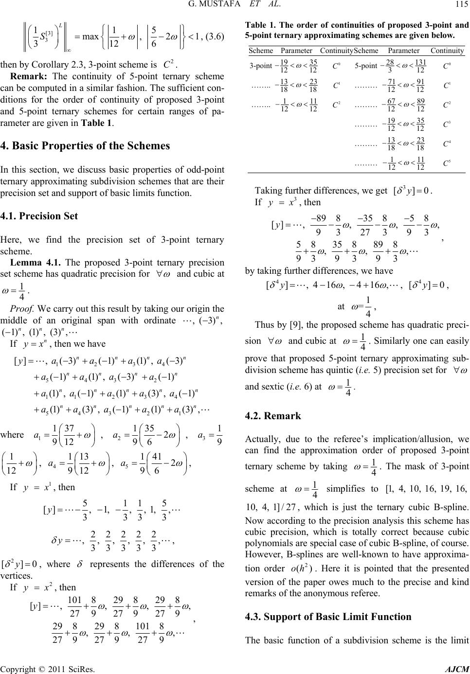

G. MUSTAFA ET AL.
115
[3]
3
115
max, 21
3126
L
S 






 
, (3.6)
then by Corollary 2.3, 3-point scheme is 2 C.
Remark: The continuity of 5-point ternary scheme
can be computed in a similar fashion. The sufficient con-
ditions for the order of continuity of proposed 3-point
and 5-point ternary schemes for certain ranges of pa-
rameter are given in Table 1.
4. Basic Properties of the Schemes
In this section, we discuss basic properties of odd-point
ternary approximating subdivision schemes that are their
precision set and support of basic limits function.
4.1. Precision Set
Here, we find the precision set of 3-point ternary
scheme.
Lemma 4.1. The proposed 3-point ternary precision
set scheme has quadratic precision for

 and cubic at
1
4
 .
Proof. We carry out this resu lt by taking ou r origin the
middle of an original span with ordinate , (3),
n

(1), (1), (3),
nn n

If n
y
x, then we have
1234
543 2
11234
543 21
[], (3)(1)(1), (3)
(1)(1), (3)(1)
(1), (1)(1)(3), (1)
(1)(3), (1)(1)(3),
nnnn
nn nn
nnnnn
nn nnn
ya aaa
aaa a
aaaa a
aaa aa
 

 
 


where 1137
912
a





, 2135 2
96
a





, 31
9
a

1
12





, 4113
912
a





, 51412
96
a





,
If 1
y
x, then
5115
[], 1, , , 1, ,
3333
y 
22222
, , , , , ,
33333
y  ,
2
[]y   , where

represents the differences of the
vertices.
If 2
y
x, then
101829 829 8
[], , , ,
27927 927 9
29 829 81018
, , ,
27 927 9279
y


 

 


,
Table 1. The order of continuities of proposed 3-point and
5-point ternary approximating schemes are given below.
Scheme Parameter ContinuityScheme Parameter Continuity
3-point19 35
12 12
  0
C 5-point 28 131
312
  0
C
…….. 1323
18 18
  1
C ……… 71 91
12 12
  1
C
…….. 111
12 12
  2
C ……… 6789
12 12
  2
C
………
19 35
12 12
  3
C
………
13 23
18 18
  4
C
………
111
12 12
  5
C
Takin g further diffe rences, we get 3
[y  .
If 3
y
x, then
898 358 58
[], , , ,
93 273 93
58 358898
, , ,
939393
y




 



,
by taking furth e r differences, we have
4
[, , ,y   , 4 [0y   ,
at 1 =4  ,
Thus by [9], the proposed scheme has quadratic preci-
sion


and cubic at 1
4


. Similarly one can easily
prove that proposed 5-point ternary approximating sub-
division scheme has quintic (i.e. 5) precision set for


and sextic (i.e. 6) at 1
4


.
4.2. Remark
Actually, due to the referee’s implication/allusion, we
can find the approximation order of proposed 3-point
ternary scheme by taking 1
4
 . The mask of 3-point
scheme at 1
4


simplifies to [1, 4, 10, 16, 19, 16,
10, 4, 1]/27, which is just the ternary cubic B-spline.
Now according to the precision analysis this scheme has
cubic precision, which is totally correct because cubic
polynomials are special case of cubic B-spline, of course.
However, B-splines are well-known to have approxima-
tion order 2 ()oh . Here it is pointed that the presented
version of the paper owes much to the precise and kind
remarks of the anonymous referee.
4.3. Support of Basic Limit Function
The basic function of a subdivision scheme is the limit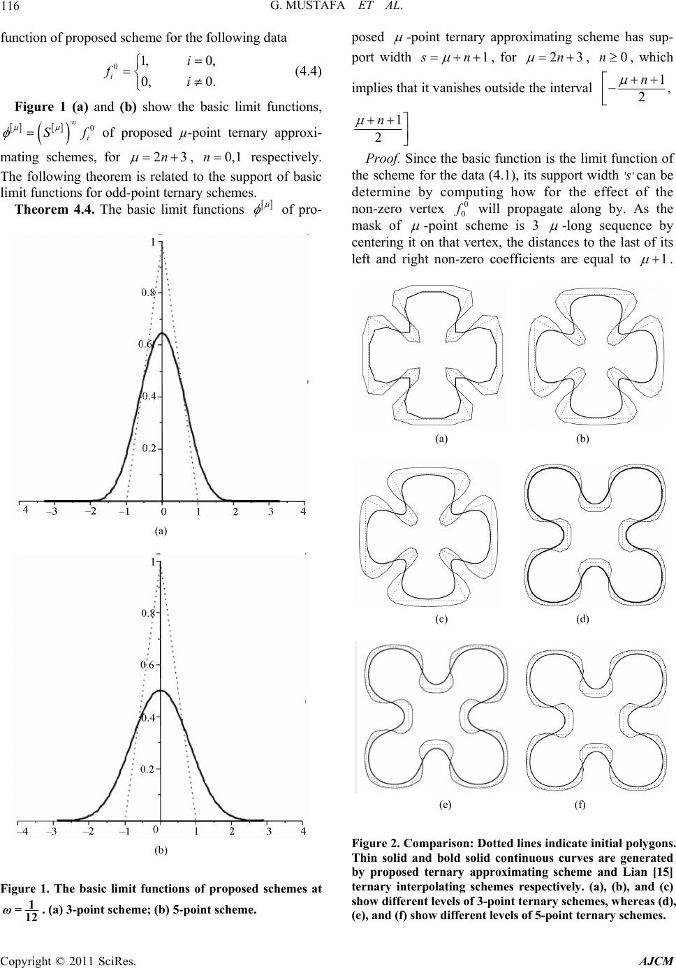

G. MUSTAFA ET AL.
116
function of proposed scheme for the following data
01, 0,
0, 0.
i
i
fi



 (4.4)
Figure 1 (a) and (b) show the basic limit functions,
 

0
i
Sf



 of proposed µ-point ternary approxi-
mating schemes, for 23n

, 0,1n respectively.
The following theorem is related to the support of basic
limit functions for odd-point ternary schemes.
Theorem 4.4. The basic limit functions



of pro-
(a)
(b)
Figure 1. The basic limit functions of proposed schemes at
1
=12 ω. (a) 3-point scheme; (b) 5-point scheme.
posed

-point ternary approximating scheme has sup-
port width 1
s
n


, for 23n

, 0n, which
implies that it vanishes outside th e interval 1,
2
n 





1
2
n 




Proof. Since the basic function is the limit function of
the scheme for the data (4.1), its support width ′s′ can be
determine by computing how for the effect of the
non-zero vertex 0
0
f
will propagate along by. As the
mask of

-point scheme is 3

-long sequence by
centering it on that vertex, the distances to the last of its
left and right non-zero coefficients are equal to 1


.
(a) (b)
(c) (d)
(e) (f)
Figure 2. Comparison: Dotted lines indicate initial polygons.
Thin solid and bold solid continuous curves are generated
by proposed ternary approximating scheme and Lian [15]
ternary interpolating schemes respectively. (a), (b), and (c)
show different levels of 3-point ternary schemes, whereas (d),
(e), and (f) show different levels of 5-point ternary schemes.

G. MUSTAFA ET AL.
117
Table 2. Comparison of proposed 3- and 5-point ternary schemes.
Scheme Type Support Order
n
C Range
3-point ternary [2] Interpolating 4 2 1 C 1
3
ab and 3
2,
99
b







3-point ternary [15] Interpolating 4 2 1
C For some particular value
3-point ternary [2] Approximating 4 2 2 C For some particular value
3-point ternary [18] Approxi mating 4 2 2
C 7
1,
72 72





4-point ternary [6] Interpolating 5 4 2
C 11
,
915




4-point ternary [4] Approximating 5.5 4 2 C For some particular value
5-point ternary [15] Interpolating 7 4 1 C For some particular value
3-point ternary proposed Approximating 4 2 2
C 111
12 12
 
5-point terna ry proposed Approximating 7 4 5 C 111
12 12
 
(a) (b)
Figure 3. Dotted lines indicate initial polygons. Dashes, dashes dot and solid line show the visual smoothness of proposed
schemes for the parametric value at -1
=12 ω, 1 =6 ω and 1 =3 ω respectively. (a) 3-point scheme; (b) 5-point scheme.
At the first subdivision step, we see that the vertices on
the both sides of 1
0
f
at 1
3
n

are the furthest non-
zero new vertices. At each refinement, the distances on
both sides are reduced by the factor 1
3. At the next step
of the scheme this will propagate along by 11
33
n




on both sides. Hence after k subdivision steps the fur-
thest non-zero vertex on the left will be at

1
20
1
11 11
1 ...
33
33 3
k
kj
j
n
n








 





. So
the total support width is

1
0
11
233
k
j
j
n 













1n.
4.4. Comparison and Application
Table 2 shows that the support size and continuity of
proposed 3-point ternary scheme is same as 3-point ter-
nary scheme introduced by [18]. It is also declared that
the scheme introduced by [18] is 2 C for


7 1,
72 72

while our 3-point scheme is 2
C for

111
,
12 12
 which
provides more freedom for curve designing. Support size
of proposed 3-point ternary approximating scheme is
smaller than 4-point ternary interpolating schemes [6]
but gives the same order of derivative continuity. It is
also mentioned that proposed 3-point scheme has larger
interval of continuity with less computational cost than
schemes [6] and [4].

G. MUSTAFA ET AL.
118
In Table 2, we have pointed out that proposed 5-point
ternary scheme is 5 C continuous while the 5-point ter-
nary scheme of [15] is 1 C.
Figure 2 shows the visual comparison of 3- and
5-point ternary interpolating schemes of Lian [15] with
the proposed 3- and 5-point ternary approximating
schemes. Figure 3 is exposed to show the role of shape
parameter

when proposed 3- and 5-point schemes
applied on discrete data points. From this figure, we see
that the behavior of the limiting curve acts as tightness
when the choice of shape parameter vary from right to
left in the interval

111
,
12 12
.
5. Conclusions
The family of odd-point approximating schemes for curve
design has established. Smoothness and approximation
order of 3- and 5-point ternary schemes have been dis-
cussed. Support of family of odd-point ternary schemes
has computed in general. It has been shown that pro-
posed schemes are better then existing odd-point ternary
schemes in the sense of smoothness. The family of
even-point ternary approximating schemes will be stud-
ied in detail in the forthcoming paper.
6. Acknowledgements
The presented version of the paper owes much to the
precise and kind remarks of the anonymous referee. This
work is supported by the Indigenous Ph. D. Scholarship
Scheme of Higher Education Commission (HEC) Paki-
stan
7. References
[1] C. Beccari, Gcasiola and L. Romani, “An Interpolating
4-Point 2
C Ternary Non-Stationary Subdivision Scheme
with Tension Control,” Computer Aided Geometric De-
sign, Vol. 24, No. 4, 2007, pp. 210-219.
doi:10.1016/j.cagd.2007.02.001
[2] M. F. Hassan, “Further Analysis of Ternary and 3-Point
Univariate Subdivision Schemes,” Technical Report 599,
University of Cambridge Computer Laboratory, ISSN
1476-2986, 2004.
[3] K. P. Ko, B.-G. Lee and G. Yoon, “A Ternary 4-Point
Approximating Subdivision Scheme,” Applied Mathemat-
ics and Computation, Vol. 190, No. 2, 2007, pp. 1563-
1573. doi:10.1016/j.amc.2007.02.032
[4] S. S. Siddiqi and K. Rehan, “Modified Form of Binary
and Ternary 3-Point Subdivision Scheme,” Applied
Mathematics and Computation, Vol. 216, No. 3, 2010, pp.
970-982. doi:10.1016/j.amc.2010.01.115
[5] M. F. Hassan, N. A. Dodgson, “Ternary and Three-Point
Univariate Subdivision Schemes,” In: A. Cohen, J. L.
Marrien, L. L. Schumaker, Eds., Curve and Surface Fit-
ting: Sant-Malo 2002, Nashboro Press, Brentwood, 2003,
pp. 199-208.
[6] M. F. Hassan, I. P. Ivrissimitzis, N. A. Dodgson and M.
A. Sabin, “An Interpolating 4-Point 2 C Ternary Sta-
tionary Subdivision Scheme,” Computer Aided Geomet-
ric Design, Vol. 19, No. 1, 2002, pp. 1-18.
doi:10.1016/S0167-8396(01)00084-X
[7] F. Khan and G. Mustafa, “Ternary Six-Point Interpolating
Subdivision Scheme,” Lobachevskii Journal of Mathe-
matics, Vol. 29, No. 3, 2008, pp. 153-163.
[8] D. Levin, “Using Laurent Polynomial Representation for
the Analysis of Non-Uniform Binary Subdivision
Schemes,” Advances in Computational Mathematics, Vol.
11, No. 1, 1999, pp. 41-54.
doi:10.1023/A:1018907522165
[9] G. Mustafa and F. Khan, “A New 4-Point 3
C Quater-
nary Approximating Subdivision Scheme,” Abstract and
Applied Analysis, Vol. 2009, 2009, Article ID 301967.
doi:10.1155/2009/301967
[10] M. Sabin, “Eigenanalysis and Artifacts of Subdivision
Curves and Surfaces, Tutorials on Multiresolution in
Geometric Modeling,” In: A. Isle, E. Quak and M. S.
Floater, Eds., Springer, Berlin, 2002, pp. 69-92.
[11] N. Dyn, K. Hormann, M. A. Sabin and Z. Shen, “Poly-
nomial Reproduction by Symmetric Subdivision
Schemes,” Journal of Approximation Theory, Vol. 155,
No. 1, 2008, pp. 28-42. doi:10.1016/j.jat.2008.04.008
[12] G. Mustafa, and A. R. Najma, “The Mask of


24b

-
Point n-ary Subdivision Scheme,” Computing, Vol. 90,
No. 1-2, 2010, pp. 1-14. doi:10.1007/s00607-010-0108-x
[13] J.-A. Lian, “On a-ary Subdivision for Curve Design: III.
2m-Point and


21m

-Point Interpolatory Schemes,”
Applications and Applied Mathematics: An International
Journal, Vol. 4, No. 2, 2009, pp. 434-444.
[14] K. Hormann and M. A. Sabin, “A Family of Subdivision
Schemes with Cubic Precision,” Computer Aided Geo-
metric Design, Vol. 25, No. 1, 2008, pp. 41-52.
doi:10.1016/j.cagd.2007.04.002
[15] A. Levin, “Polynomial Generation and Quasi-Interpolation
in Stationary and Non-Uniform Subdivision Schemes,”
Computer Aided Geometric Design, Vol. 20, No. 1, 2003,
pp. 41-60. doi:10.1016/S0167-8396(03)00006-2
[16] J.-A. Lian, “On a-ary Subdivision for Curve Design: II.
3-Point and 5-Point Interpolatory Schemes,” Applications
and Applied Mathematics: An International Journal, Vol.
3, No. 2, 2008, pp. 176-187.
[17] Y. Tang, K. P. Ko and B.-G. Lee, “A New Proof of
Smoothness of 4-Point Deslauriers-Dubic Scheme,”
Journal of Applied Mathematics and Computing, Vol. 18,
No. 1-2, 2005, pp. 553-562.
[18] J.-A. Lian, “On a-ary Subdivision for Curve Design: I.
4-Point and 6-Point Interpolatory Schemes,” Applications
and Applied Mathematics: An International Journal, Vol.
3, No. 1, 2008, pp. 18-29.