 Journal of Modern Physics, 2011, 2, 472-480 doi:10.4236/jmp.2011.26057 Published Online June 2011 (http://www.SciRP.org/journal/jmp) Copyright © 2011 SciRes. JMP Study of the Double Nonlinear Quantum Resonances in Diatomic Molecules Gustavo López, Jorge Gomez Tejeda Zanudo Departamento de Físic a, Uni versidad de Guad al ajara, Guadalajara, Mexico E-mail: gulopez@udgserv.cencar.udg.m x, jgtz.fis@gmail.com Received February 23, 2011; revised March 29, 2011; accepted April 19, 2011 Abstract We study the quantum dynamics of diatomic molecule driven by a circularly polarized resonant electric field. We look for a quantum effect due to classical chaos appearing due to the overlapping of nonlinear reso- nances associated to the vibrational and rotational motion. We solve the Schrödinger equation associated with the wave function expanded in term of proper stationary states, nlm (vibrational angular momentum states). Looking for quantum-classic correspondence, we consider the Liouville dynamics in the two dimensional phase space defined by the coherent-like state of vibrational states. We consider the rela- tionship between the overlapping of the classical resonances and the mixing of the quantum states, and it is found some similarities when the quantum dynamics is pictured in terms of number and phase operators. Keywords: Nonlinear Resonance, Diatomic Molecule, Quantum Resonances 1. Introduction The study of quantum dynamics in the interval of pa- rameters where classical chaotic behavior occurs is what we call “Quantum Chaos, Chaology, or Quantum Mani- festation of Chaos” [1] which deals with some type of quantum manifestation of the classical chaos, mainly associated with the statistical properties of near neighbor levels of energy of the system [1]. In contrast, for quan- tum systems associated to non chaotic classical ones, it is mostly believed that classical dynamical behavior must occur for large quantum numbers or high value of the action variable [2] (Rydberg states). In particular, studies of dynamical chaos in atomic and molecular systems has been of great theoretical and practical interest [3-12] since not enough integrals of motion are found either in the classical or in its quantum system. Different ap- proaches and studies have been used for the classical [13-15] and quantum (quasi-classical region) [16-18] cases, and most of them are based on the Morse potential as the inter-atomic interaction [19]. On the other hand, the classical study of the dynamics of atomic and mo- lecular systems has shown that, under certain conditions, these systems are capable of exhibiting a chaotic behav- ior, even in the case the system has few degrees of free- dom. In what follows of this introduction and to have a better perspective of the problem, we summarize what Berman et al. [20] did for the classical part of the prob- lem. It is known that the dynamics of a diatomic molecule in a resonant circularly polarized electric field can be modeled by the Hamiltonian 00 ,; ,; ,=,,; , ,,, vib rot int HI ppHIHpp HI t (1) where describes the vibration of the molecule along its axis in terms of the action variable I and its conjugated angle variable () 0vib H , describes the rota- tion of the molecule around its transversal axis of sym- metry in terms of spherical coordinates ( () 0rot H ,,r ), and = int tdE describes the interaction of the electric dipole moment (d) of the molecule with and external electric field ( tE). These term are given explicitly by () 2 0 2 () 2 022 ,= , 1 ,; ,=, 2sin vib eee rot HI IxI p Hppp r (2) and 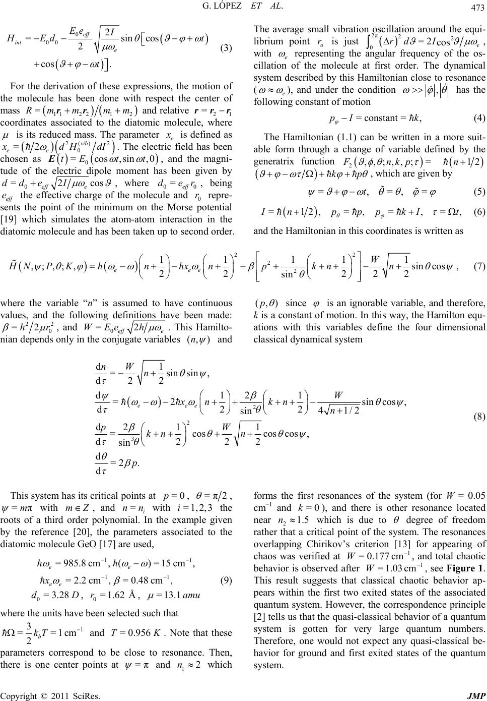 G. LÓPEZ ET AL. 473 0 00 2 =sincos 2 cos . eff int e Ee I Ed t t (3) For the derivation of these expressions, the motion of the molecule has been done with respect the center of mass 11 221 2 =Rm mmmrr and relative 21 = rrr coordinates associated to the diatomic molecule, where is its reduced mass. The parameter e is defined as 2() 2 0 =2 vib ee dH dI . The electric field has been chosen as , and the magni- tude of the electric dipole moment has been given by 0 =cos,sin,0tEt t E 0 =2c eff e dd eIos , where 0eff , being eff the effective charge of the molecule and 0 repre- sents the point of the minimum on the Morse potential [19] which simulates the atom-atom interaction in the diatomic molecule and has been taken up to second order. The average small vibration oscillation around the equi- librium point o is just 0 r r =de e r 2π22 0e =2 cos rd I , with e representing the angular frequency of the os- cillation of the molecule at first order. The dynamical system described by this Hamiltonian close to resonance (e ), and under the condition , has the following constant of motion =constant= ,pI k (4) The Hamiltonian (1.1) can be written in a more suit- able form through a change of variable defined by the generatrix function 2,,;,,;=Fnkp 12n kp = , which are given by =,=,t (5) =12,=,=,=, npppkI t (6) and the Hamiltonian in this coordinates is written as 22 2 2 11 111 ,;,;, sin cos 22 222 sin eee W HNPKnxnpk nn , (7) where the variable “n” is assumed to have continuous values, and the following definitions have been made: 2 0 =2r2 , and 0 =2 eff e WEe . This Hamilto- nian depends only in the conjugate variables (, )n and (,)p since is an ignorable variable, and therefore, k is a constant of motion. In this way, the Hamilton equ- ations with this variables define the four dimensional classical dynamical system 2 2 3 d1 =sinsin, d22 d121 =2 sinc d22 41/2 sin d2 11 =coscoscos, d222 sin d=2 . d eee nW n W xnknn pW kn n p os, (8) This system has its critical points at , =0p=π2 , =πm with , and with the roots of a third order polynomial. In the example given by the reference [20], the parameters associated to the diatomic molecule GeO [17] are used, mZ=i nn =1i,2,3 1 =985.8cm,()= 15cm, ee 1 1 1 =2.2 cm,=0.48 cm, ee x (9) 0=3.28dD, , 0=1.62rÅ= 13.1 amu where the units have been selected such that 1 3 ==1cm 2b kT and . Note that these =0.956TK parameters correspond to be close to resonance. Then, there is one center points at =π and which forms the first resonances of the system (for W = 0.05 cm–1 and ), and there is other resonance located near 2 12n =0k 1.5n which is due to degree of freedom rather that a critical point of the system. The resonances overlapping Chirikov’s criterion [13] for appearing of chaos was verified at , and total chaotic behavior is observed after , see Figure 1. This result suggests that classical chaotic behavior ap- pears within the first two exited states of the associated quantum system. However, the correspondence principle [2] tells us that the quasi-classical behavior of a quantum system is gotten for very large quantum numbers. Therefore, one would not expect any quasi-classical be- havior for ground and first exited states of the quantum system. 1 = 0.177W =1 cmW cm .03 1 Copyright © 2011 SciRes. JMP 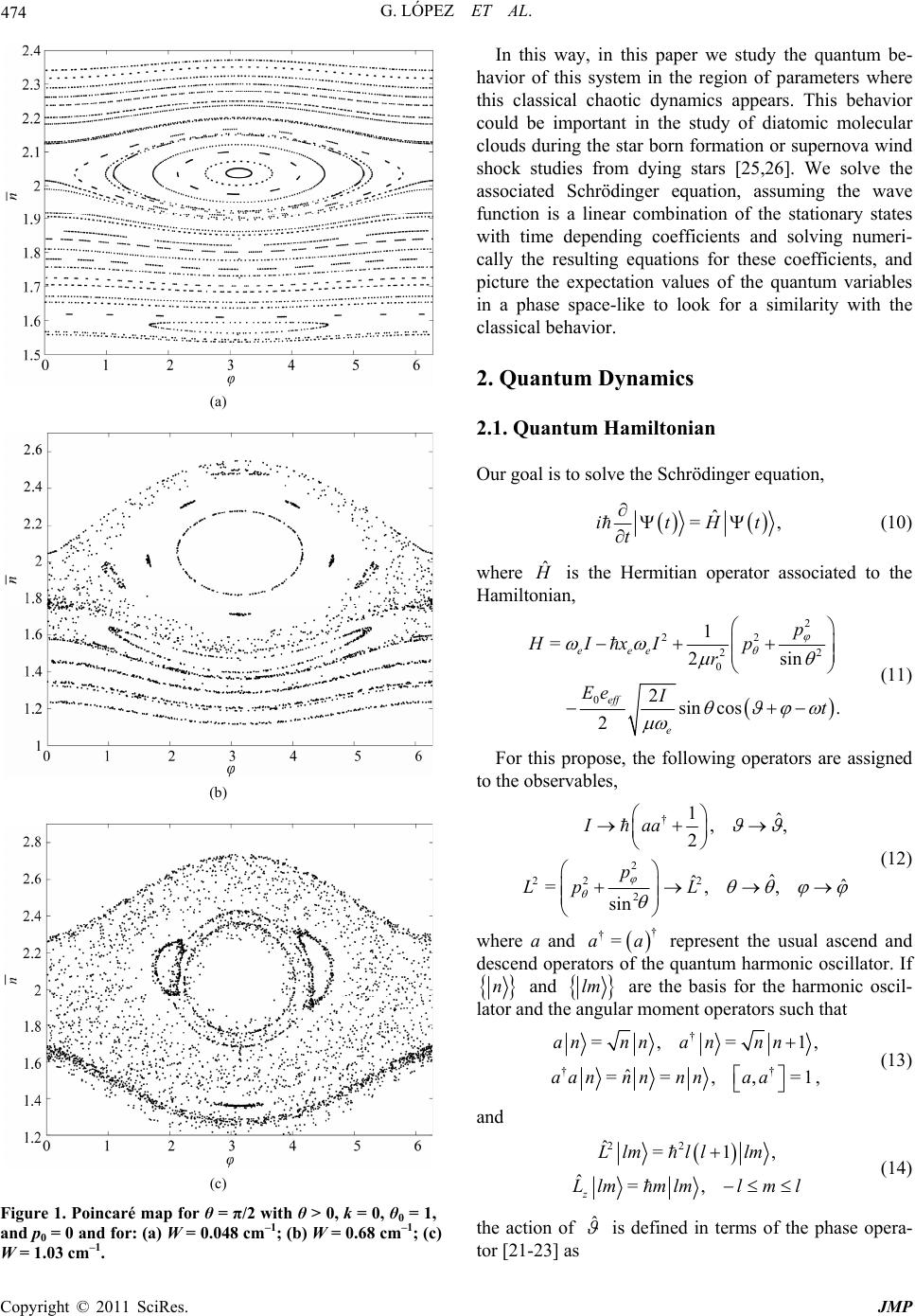 474 G. LÓPEZ ET AL. (a) (b) (c) Figure 1. Poincaré map for θ = π/2 with θ > 0, k = 0, θ0 = 1, and p0 = 0 and for: (a) W = 0.048 cm–1; (b) W = 0.68 cm–1; (c) W = 1.03 cm–1. In this way, in this paper we study the quantum be- havior of this system in the region of parameters where this classical chaotic dynamics appears. This behavior could be important in the study of diatomic molecular clouds during the star born formation or supernova wind shock studies from dying stars [25,26]. We solve the associated Schrödinger equation, assuming the wave function is a linear combination of the stationary states with time depending coefficients and solving numeri- cally the resulting equations for these coefficients, and picture the expectation values of the quantum variables in a phase space-like to look for a similarity with the classical behavior. 2. Quantum Dynamics 2.1. Quantum Hamiltonian Our goal is to solve the Schrödinger equation, ˆ =itHt t , (10) where ˆ is the Hermitian operator associated to the Hamiltonian, 2 22 22 0 0 1 =2sin 2sin cos. 2 eee eff e p HIxI p r Ee It (11) For this propose, the following operators are assigned to the observables, † 2 22 2 2 1ˆ ,, 2 ˆ ˆˆ =,, sin Iaa p Lp L (12) where a and represent the usual ascend and descend operators of the quantum harmonic oscillator. If † †=aa n and lm are the basis for the harmonic oscil- lator and the angular moment operators such that † †† =,= 1 ˆ ==,,=1 an nnan nn aannnnn aa , , (13) and 22 ˆ=1, ˆ=, z Llmll lm Llmmlmlml (14) the action of ˆ is defined in terms of the phase opera- tor [21-23] as Copyright © 2011 SciRes. JMP 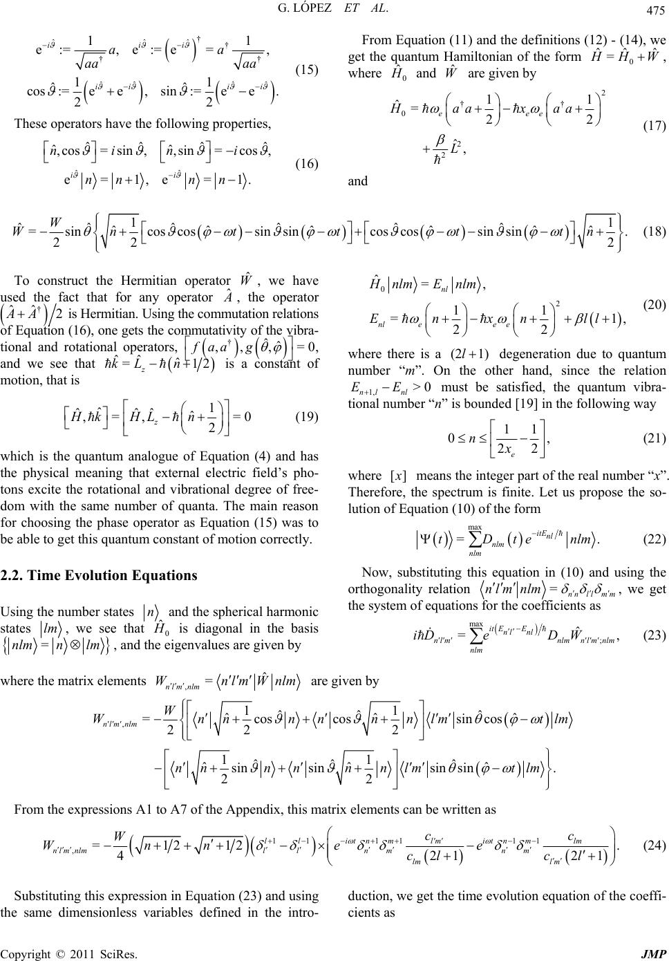 G. LÓPEZ ET AL. Copyright © 2011 SciRes. JMP 475 † ˆˆˆ † † ˆˆ ˆˆ 1 e:=,e:=e =, 11 ˆˆ cos:=e e,sin:=e e 22 iii ii ii aa aa aa † 1 . (15) From Equation (11) and the definitions (12) - (14), we get the quantum Hamiltonian of the form 0 ˆˆ ˆ = HW , where 0 ˆ and are given by ˆ W 2 †† 0 2 2 11 ˆ=22 ˆ, eee Haaxaa L These operators have the following properties, (17) ˆˆ ˆˆ ˆ ˆˆ ,cos=sin,,sin=cos, e=1,e =1. ii nin i nn nn ˆ (16) and 1 1 ˆˆ ˆˆ ˆ ˆˆˆ ˆˆ ˆ ˆ =sincos cossin sincos cossin sin. 22 2 W Wnt tt tn (18) To construct the Hermitian operator , we have used the fact that for any operator ˆ W ˆ , the operator † ˆˆ 2AA is Hermitian. Using the commutation relations of Equation (16), one gets the commutativity of the vibra- tional and rotational operators, , and we see that ,, g ˆˆ , =fa † a0 ˆˆˆ = z kL n 1 2 is a constant of motion, that is 0 2 ˆ=, 11 =1 22 nl nlee e H nlmEnlm Enxn ll , (20) where there is a (2 1)l degeneration due to quantum number “m”. On the other hand, since the relation 1, >0 nl nl EE must be satisfied, the quantum vibra- tional number “n” is bounded [19] in the following way 1 ˆ ˆˆˆ ˆ ,=, = 2 z Hk HLn 0 (19) 11 0 22 e nx, (21) which is the quantum analogue of Equation (4) and has the physical meaning that external electric field’s pho- tons excite the rotational and vibrational degree of free- dom with the same number of quanta. The main reason for choosing the phase operator as Equation (15) was to be able to get this quantum constant of motion correctly. where [] means the integer part of the real number “x”. Therefore, the spectrum is finite. Let us propose the so- lution of Equation (10) of the form max = . (22) itEnl nlm nlm tDtenlm Now, substituting this equation in (10) and using the orthogonality relation =nnll mm nlm nlm , we get the system of equations for the coefficients as 2.2. Time Evolution Equations Using the number states n and the spherical harmonic states lm , we see that 0 ˆ is diagonal in the basis max ; ˆ =, it EE nl nl nlmnlmnlm nlm nlm iDeD W (23) =nlm n lm, and the eigenvalues are given by where the matrix elements ,ˆ = nlm nlm WnlmWn lm are given by , 11 ˆˆ ˆ ˆ ˆˆ =coscossin cos 22 2 11 ˆˆ ˆ ˆ ˆˆ sinsinsin sin. 22 nlm nlmW Wnnnnnnlm nnn nnnlmtlm tlm From the expressions A1 to A7 of the Appendix, this matrix elements can be written as 11 1111 ,=1212 421 llitnmit nm lm lm nlm nlmllnmnm lmlm cc W Wnnee clc l . 21 (24) Substituting this expression in Equation (23) and using the same dimensionless variables defined in the intro- duction, we get the time evolution equation of the coeffi- cients as 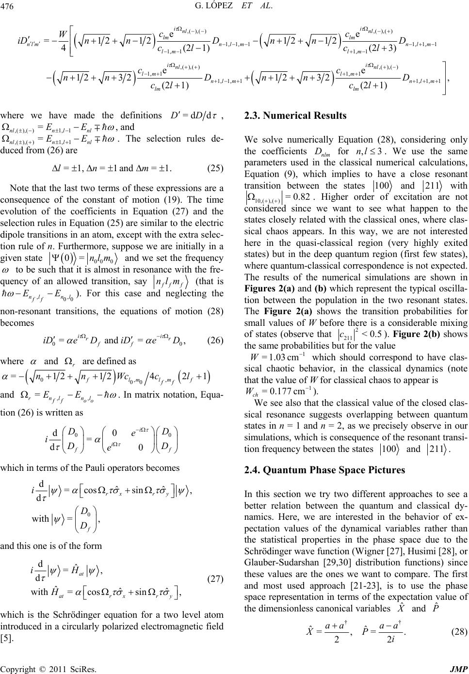 476 G. LÓPEZ ET AL. ,( ),( ),( ),() 1, 1,11, 1,1 1, 11, 1 ,( ),(), 1, 11, 1 1, 1,1 ee =1212 1212 4(21) (23) ee 12 3212 32 (2 1) ii nl nl lm lm nlmn lmn lm lm lm i i nl nl lm lm nlm lm cc W iDnnDn nD cl cl cc nnD nn cl (),() 1, 1,1, (2 1)nlm lm D cl where we have made the definitions =d dDD , ,( ),( )1,1 = nln lnl EE =EE, and ,( ),( )1,1nln lnl . The selection rules de- duced from (26) are =1, =1and=1.ln m (25) Note that the last two terms of these expressions are a consequence of the constant of motion (19). The time evolution of the coefficients in Equation (27) and the selection rules in Equation (25) are similar to the electric dipole transitions in an atom, except with the extra selec- tion rule of n. Furthermore, suppose we are initially in a given state 00 0 0=nlm and we set the frequency to be such that it is almost in resonance with the fre- quency of an allowed transition, say ff nlm (that is , 00 nl nl ff EE , ). For this case and neglecting the non-resonant transitions, the equations of motion (28) becomes 0 =and= ii r ff iDe DiDeD 0 , r (26) where and are defined as r 0,, 00 =121242 flmlmf ff nnWccl 1 and ,, = rnl nl ff oo EE . In matrix notation, Equa- tion (26) is written as 0 0 d= d0 i i 0 f D e iD e D D which in terms of the Pauli operators becomes 0 dˆˆ =cossin d with =, rx ry f i D D , and this one is of the form dˆ =, d ˆˆˆ with= cossin, at atrxry iH H 3 (27) which is the Schrödinger equation for a two level atom introduced in a circularly polarized electromagnetic field [5]. 2.3. Numerical Results We solve numerically Equation (28), considering only the coefficients nlm for . We use the same parameters used in the classical numerical calculations, Equation (9), which implies to have a close resonant transition between the states D,nl 100 and 211 with 10,( ),( )=0.82 . Higher order of excitation are not considered since we want to see what happen to the states closely related with the classical ones, where clas- sical chaos appears. In this way, we are not interested here in the quasi-classical region (very highly exited states) but in the deep quantum region (first few states), where quantum-classical correspondence is not expected. The results of the numerical simulations are shown in Figures 2(a) and (b) which represent the typical oscilla- tion between the population in the two resonant states. The Figure 2(a) shows the transition probabilities for small values of W before there is a considerable mixing of states (observe that 2 211 <0.5c). Figure 2(b) shows the same probabilities but for the value 1 =1.03 cmW which should correspond to have clas- sical chaotic behavior, in the classical dynamics (note that the value of W for classical chaos to appear is 1 =0.177 cm ch W ). We see also that the classical value of the closed clas- sical resonance suggests overlapping between quantum states in n = 1 and n = 2, as we precisely observe in our simulations, which is consequence of the resonant transi- tion frequency between the states 100 and 211. 2.4. Quantum Phase Space Pictures In this section we try two different approaches to see a better relation between the quantum and classical dy- namics. Here, we are interested in the behavior of ex- pectation values of the dynamical variables rather than the statistical properties in the phase space due to the Schrödinger wave function (Wigner [27], Husimi [28], or Glauber-Sudarshan [29,30] distribution functions) since these values are the ones we want to compare. The first and most used approach [21-23], is to use the phase space representation in terms of the expectation value of the dimensionless canonical variables ˆ and ˆ P †† ˆˆ =,= 22 aa aa XP i . (28) Copyright © 2011 SciRes. JMP 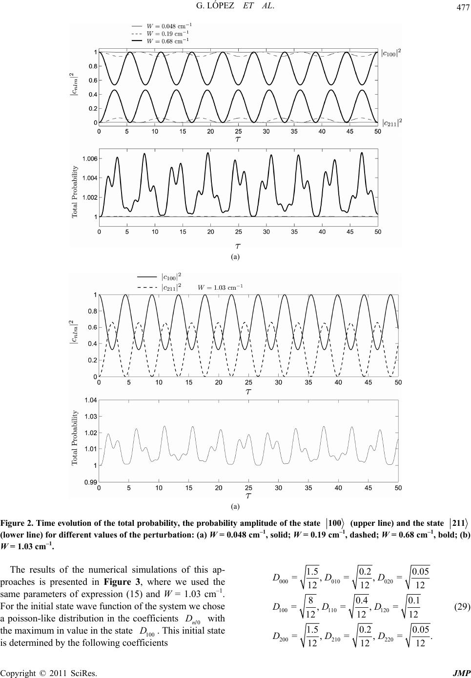 G. LÓPEZ ET AL. 477 (a) (a) Figure 2. Time evolution of the total probability, the probability amplitude of the state 100 (upper line) and the state 211 (lower line) for different values of the perturbation: (a) W = 0.048 cm–1, solid; W = 0.19 cm–1, dashed; W = 0.68 cm–1, bold; (b) W = 1.03 cm–1. The results of the numerical simulations of this ap- proaches is presented in Figure 3, where we used the same parameters of expression (15) and W = 1.03 cm–1. For the initial state wave function of the system we chose a poisson-like distribution in the coefficients with the maximum in value in the state . This initial state is determined by the following coefficients 0nl D 100 D 000 010020 100 110120 200 210220 1.5 0.2 0.05 =,=,= 12 1212 80.40. =,=,= 12 1212 1.5 0.2 0.05 =,=,= 12 1212 DDD DD D DDD 1 . (29) Copyright © 2011 SciRes. JMP 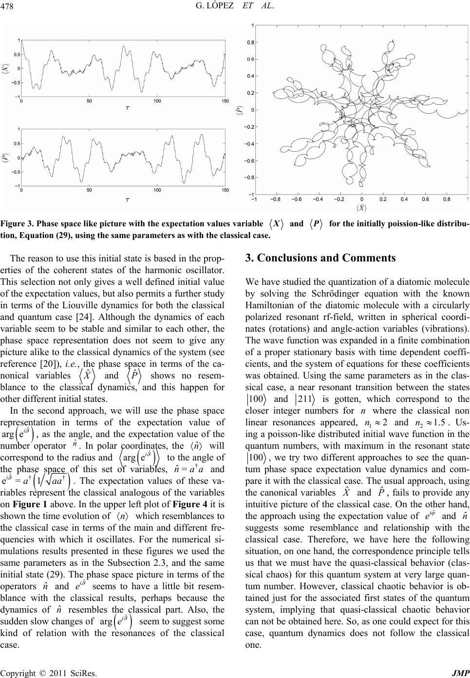 478 G. LÓPEZ ET AL. Figure 3. Phase space like picture with the expectation values variable and for the initially poission-like distribu- tion, Equation (29), using the same parameters as with the classical case. The reason to use this initial state is based in the prop- erties of the coherent states of the harmonic oscillator. This selection not only gives a well defined initial value of the expectation values, but also permits a further study in terms of the Liouville dynamics for both the classical and quantum case [24]. Although the dynamics of each variable seem to be stable and similar to each other, the phase space representation does not seem to give any picture alike to the classical dynamics of the system (see reference [20]), i.e., the phase space in terms of the ca- nonical variables ˆ and ˆ P shows no resem- blance to the classical dynamics, and this happen for other different initial states. In the second approach, we will use the phase space representation in terms of the expectation value of ˆ arg ei , as the angle, and the expectation value of the number operator . In polar coordinates, the n ˆˆ n will correspond to the radius and ˆ arg ei to the angle of the phase space of this set of variables, and † na a ˆ= ˆ e= ia † a 3. Conclusions and Comments We have studied the quantization of a diatomic molecule by solving the Schrödinger equation with the known Hamiltonian of the diatomic molecule with a circularly polarized resonant rf-field, written in spherical coordi- nates (rotations) and angle-action variables (vibrations). The wave function was expanded in a finite combination of a proper stationary basis with time dependent coeffi- cients, and the system of equations for these coefficients was obtained. Using the same parameters as in the clas- sical case, a near resonant transition between the states 100 and 211 is gotten, which correspond to the closer integer numbers for where the classical non linear resonances appeared, 1 and 2 nn21.5n . Us- ing a poisson-like distributed initial wave function in the quantum numbers, with maximum in the resonant state 100 , we try two different approaches to see the quan- tum phase space expectation value dynamics and com- pare it with the classical case. The usual approach, using the canonical variables ˆ and , fails to provide any intuitive picture of the classical case. On the other hand, the approach using the expectation value of ˆ P ˆ i e and suggests some resemblance and relationship with the classical case. Therefore, we have here the following situation, on one hand, the correspondence principle tells us that we must have the quasi-classical behavior (clas- sical chaos) for this quantum system at very large quan- tum number. However, classical chaotic behavior is ob- tained just for the associated first states of the quantum system, implying that quasi-classical chaotic behavior can not be obtained here. So, as one could expect for this case, quantum dynamics does not follow the classical one. ˆ n † 1a . The expectation values of these va- riables represent the classical analogous of the variables on Figure 1 above. In the upper left plot of Figure 4 it is shown the time evolution of n which resemblances to the classical case in terms of the main and different fre- quencies with which it oscillates. For the numerical si- mulations results presented in these figures we used the same parameters as in the Subsection 2.3, and the same initial state (29). The phase space picture in terms of the operators and ˆ ˆ ni e seems to have a little bit resem- blance with the classical results, perhaps because the dynamics of resembles the classical part. Also, the sudden slow changes of ˆ n ˆ i e arg seem to suggest some kind of relation with the resonances of the classical case. Copyright © 2011 SciRes. JMP 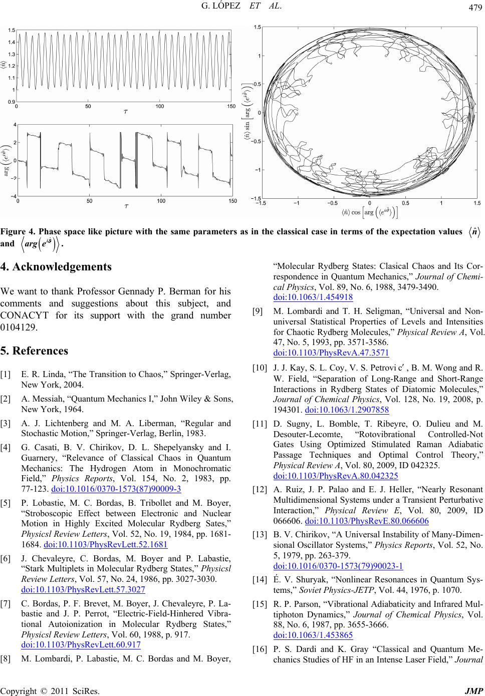 G. LÓPEZ ET AL. Copyright © 2011 SciRes. JMP 479 Figure 4. Phase space like picture with the same parameters as in the classical case in terms of the expectation values ˆ n and ˆ i arg e . 4. Acknowledgements We want to thank Professor Gennady P. Berman for his comments and suggestions about this subject, and CONACYT for its support with the grand number 0104129. 5. References [1] E. R. Linda, “The Transition to Chaos,” Springer-Verlag, New York, 2004. [2] A. Messiah, “Quantum Mechanics I,” John Wiley & Sons, New York, 1964. [3] A. J. Lichtenberg and M. A. Liberman, “Regular and Stochastic Motion,” Springer-Verlag, Berlin, 1983. [4] G. Casati, B. V. Chirikov, D. L. Shepelyansky and I. Guarnery, “Relevance of Classical Chaos in Quantum Mechanics: The Hydrogen Atom in Monochromatic Field,” Physics Reports, Vol. 154, No. 2, 1983, pp. 77-123. doi:10.1016/0370-1573(87)90009-3 [5] P. Lobastie, M. C. Bordas, B. Tribollet and M. Boyer, “Stroboscopic Effect between Electronic and Nuclear Motion in Highly Excited Molecular Rydberg Sates,” Physicsl Review Letters, Vol. 52, No. 19, 1984, pp. 1681- 1684. doi:10.1103/PhysRevLett.52.1681 [6] J. Chevaleyre, C. Bordas, M. Boyer and P. Labastie, “Stark Multiplets in Molecular Rydberg States,” Physicsl Review Letters, Vol. 57, No. 24, 1986, pp. 3027-3030. doi:10.1103/PhysRevLett.57.3027 [7] C. Bordas, P. F. Brevet, M. Boyer, J. Chevaleyre, P. La- bastie and J. P. Perrot, “Electric-Field-Hinhered Vibra- tional Autoionization in Molecular Rydberg States,” Physicsl Review Letters, Vol. 60, 1988, p. 917. doi:10.1103/PhysRevLett.60.917 [8] M. Lombardi, P. Labastie, M. C. Bordas and M. Boyer, “Molecular Rydberg States: Clasical Chaos and Its Cor- respondence in Quantum Mechanics,” Journal of Chemi- cal Physics, Vol. 89, No. 6, 1988, 3479-3490. doi:10.1063/1.454918 [9] M. Lombardi and T. H. Seligman, “Universal and Non- universal Statistical Properties of Levels and Intensities for Chaotic Rydberg Molecules,” Physical Review A, Vol. 47, No. 5, 1993, pp. 3571-3586. doi:10.1103/PhysRevA.47.3571 [10] J. J. Kay, S. L. Coy, V. S. Petrovic, B. M. Wong and R. W. Field, “Separation of Long-Range and Short-Range Interactions in Rydberg States of Diatomic Molecules,” Journal of Chemical Physics, Vol. 128, No. 19, 2008, p. 194301. doi:10.1063/1.2907858 [11] D. Sugny, L. Bomble, T. Ribeyre, O. Dulieu and M. Desouter-Lecomte, “Rotovibrational Controlled-Not Gates Using Optimized Stimulated Raman Adiabatic Passage Techniques and Optimal Control Theory,” Physical Review A, Vol. 80, 2009, ID 042325. doi:10.1103/PhysRevA.80.042325 [12] A. Ruiz, J. P. Palao and E. J. Heller, “Nearly Resonant Multidimensional Systems under a Transient Perturbative Interaction,” Physical Review E, Vol. 80, 2009, ID 066606. doi:10.1103/PhysRevE.80.066606 [13] B. V. Chirikov, “A Universal Instability of Many-Dimen- sional Oscillator Systems,” Physics Reports, Vol. 52, No. 5, 1979, pp. 263-379. doi:10.1016/0370-1573(79)90023-1 [14] É. V. Shuryak, “Nonlinear Resonances in Quantum Sys- tems,” Soviet Physics-JETP, Vol. 44, 1976, p. 1070. [15] R. P. Parson, “Vibrational Adiabaticity and Infrared Mul- tiphoton Dynamics,” Journal of Chemical Physics, Vol. 88, No. 6, 1987, pp. 3655-3666. doi:10.1063/1.453865 [16] P. S. Dardi and K. Gray “Classical and Quantum Me- chanics Studies of HF in an Intense Laser Field,” Journal  480 G. LÓPEZ ET AL. of Chemical Physics, Vol. 77, No. 3, 1982, 1345-1353. doi:10.1063/1.443957 [17] G. P. Berman and A. R. Kolovsky, “Quantum Chaos in a Diatomic Molecule Interacting with a Resonant Field,” Soviet Physics-JETP, Vol. 68, 1989, p. 898. [18] G. P. Berman and A. R. Kolovsky, “Quantum Chaos in Interactions of Multilevel Quantum Systems with a Co- herent Radiation Field,” Soviet Physics-USP, Vol. 35, No. 4, 1992, p. 303. [19] P. M. Morse, “Diatomic Molecules According to the Wave Mechanics II. Vibrational Lavels,” Physical Re- view, Vol. 34, No. 1, 1929, pp. 57-64. [20] G. P. Berman, E. N. Bulgakov and D. D. Holm, “Nonlin- ear Resonance and Dynamical Chaos in a Diatomic Molecule Driven by a Resonant RF Field,” Physical Re- view A, Vol. 52, 1995, p. 3074. doi:10.1103/PhysRevA.52.3074 [21] L. Susskind and J. Glogower, “Quantum Mechanical Phase and Time Operator,” Physics, Vol. 1, 1964, pp. 49-61. [22] A. Lahiri, G. Ghosh and T. K. Kar, “Action-Angle Vari- ables in Quantum Mechanics,” Physical Letters A, Vol. 238, No. 4-5, 1998, 239-243. doi:10.1016/S0375-9601(97)00926-2 [23] P. Carruthers and M. M. Nieto, “Phase and Angle Vari- ables in Quantum Mechanics,” Reviews of Modern Phys- ics, Vol. 40, No. 2, 1968, pp. 411-440. doi:10.1103/RevModPhys.40.411 [24] G. J. Milburn, “Quantum and Classical Liouville Dy- namics of the Anharmonic Oscillator,” Physical Reviews A, Vol. 33, No. 1, 1980, pp. 674-685. doi:10.1103/PhysRevA.33.674 [25] M. Burton, “IC-443-The Interaction of a Supernova Rem- nant with a Molecular Cloud,” Royal Astronomical Soci- ety, Vol. 28, 1987, pp. 269-276. [26] R. Chevalier, “Supernova Remnants in Molecular- Clouds,” Astrophysical Journal 511, 798 (1999). doi:10.1086/306710 [27] E. Wigner, “On the Quantum Correction for Thermody- namic Equilibrium,” Physical Review, Vol. 40, No. 5, 1932, pp. 749-759. doi:10.1103/PhysRev.40.749 [28] K. Husimi, “Some Formal Properties of the Density Ma- trix,” Journal of the Physical Society of Japan, Vol. 22, No. 4, 1940, pp. 264-314. [29] R. J. Glauber, “Coherent and Incoherent States of the Radiation Field,” Physical Review, Vol. 131, No. 6, 1963, pp. 2766-2788. doi:10.1103/PhysRev.131.2766 [30] E. C. G. Sudarshan, “Equivalence of Semiclassical and Quantum Mechanical Descriptions of Statistical Light Beams,” Physical Review Letters, Vol. 10, No. 7, 1963, 277-279. Copyright © 2011 SciRes. JMP
|