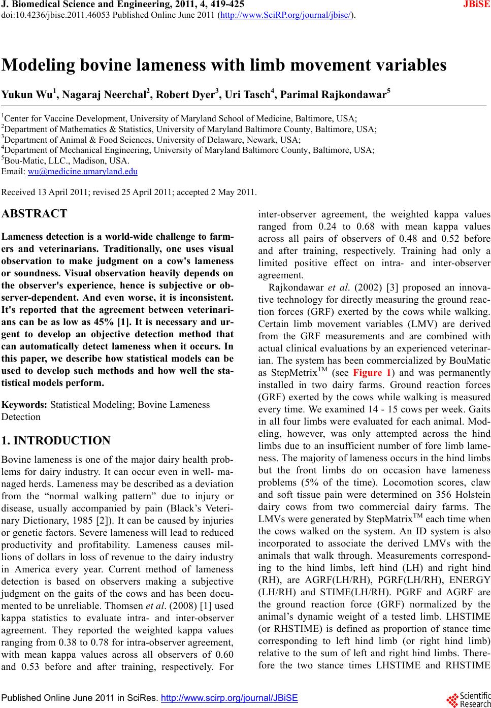J. Biomedical Science and Engineering, 2011, 4, 419-425 JBiSE
doi:10.4236/jbise.2011.46053 Published Online June 2011 (http://www.SciRP.org/journal/jbise/).
Published Online June 2011 in SciRes. http://www.scirp.org/journal/JBiSE
Modeling bovine lameness with limb movement variables
Yu kun Wu1, N a ga r a j Nee rcha l2, Robert Dyer3, Uri Tasch4, Parimal Rajkondawar5
1Center for Vaccine Development, University of Maryland School of Medicine, Baltimore, USA;
2Department of Mathematics & Statistics, University of Maryland Baltimore County, Baltimore, USA;
3Department of Animal & Food Sciences, University of Delaware, Newark, USA;
4Department of Mechanical Engineering, University of Maryland Baltimore County, Baltimore, USA;
5Bou-Matic, LLC., Madison, USA.
Received 13 April 2011; revised 25 April 2011; accepted 2 May 2011.
ABSTRACT
Lameness detection is a world-wide challenge to farm-
ers and veterinarians. Traditionally, one uses visual
observation to make judgment on a cow's lameness
or soundness. Visual observation heavily depends on
the observer's experience, hence is subjective or ob-
server-dependent. And even worse, it is inconsistent.
It's reported that the agreement between veterinari-
ans can be as low as 45% [1]. It is necessary and ur-
gent to develop an objective detection method that
can automatically detect lameness when it occurs. In
this paper, we describe how statistical models can be
used to develop such methods and how well the sta-
tistical models perform.
Keywords: Statistical Modeling; Bovine Lameness
Detection
1. INTRODUCTION
Bovine lameness is one of the major dairy health prob-
lems for dairy industry. It can occur even in well- ma-
naged herds. Lameness may be described as a deviation
from the “normal walking pattern” due to injury or
disease, usually accompanied by pain (Black’s Veteri-
nary Dictionary, 1985 [2]). It can be caused by injuries
or genetic factors. Severe lameness will lead to reduced
productivity and profitability. Lameness causes mil-
lions of dollars in loss of revenue to the dairy industry
in America every year. Current method of lameness
detection is based on observers making a subjective
judgment on the gaits of the cows and has been docu-
mented to be unreliable. Thomsen et al. (2008) [1] used
kappa statistics to evaluate intra- and inter-observer
agreement. They reported the weighted kappa values
ranging from 0.38 to 0.78 for intra-observer agreement,
with mean kappa values across all observers of 0.60
and 0.53 before and after training, respectively. For
inter-observer agreement, the weighted kappa values
ranged from 0.24 to 0.68 with mean kappa values
across all pairs of observers of 0.48 and 0.52 before
and after training, respectively. Training had only a
limited positive effect on intra- and inter-observer
agreement.
Rajkondawar et al. (2002) [3] proposed an innova-
tive technology for directly measuring the ground reac-
tion forces (GRF) exerted by the cows while walking.
Certain limb movement variables (LMV) are derived
from the GRF measurements and are combined with
actual clinical evaluations by an experienced veterinar-
ian. The system has been commercialized by BouMatic
as StepMetrixTM (see Figure 1) and was permanently
installed in two dairy farms. Ground reaction forces
(GRF) exerted by the cows while walking is measured
every time. We examined 14 - 15 cows per week. Gaits
in all four limbs were evaluated for each animal. Mod-
eling, however, was only attempted across the hind
limbs due to an insufficient number of fore limb lame-
ness. The majority of lameness occurs in the hind limbs
but the front limbs do on occasion have lameness
problems (5% of the time). Locomotion scores, claw
and soft tissue pain were determined on 356 Holstein
dairy cows from two commercial dairy farms. The
LMVs were generated by StepMatrixTM each time when
the cows walked on the system. An ID system is also
incorporated to associate the derived LMVs with the
animals that walk through. Measurements correspond-
ing to the hind limbs, left hind (LH) and right hind
(RH), are AGRF(LH/RH), PGRF(LH/RH), ENERGY
(LH/RH) and STIME(LH/RH). PGRF and AGRF are
the ground reaction force (GRF) normalized by the
animal’s dynamic weight of a tested limb. LHSTIME
(or RHSTIME) is defined as proportion of stance time
corresponding to left hind limb (or right hind limb)
relative to the sum of left and right hind limbs. There-
fore the two stance times LHSTIME and RHSTIME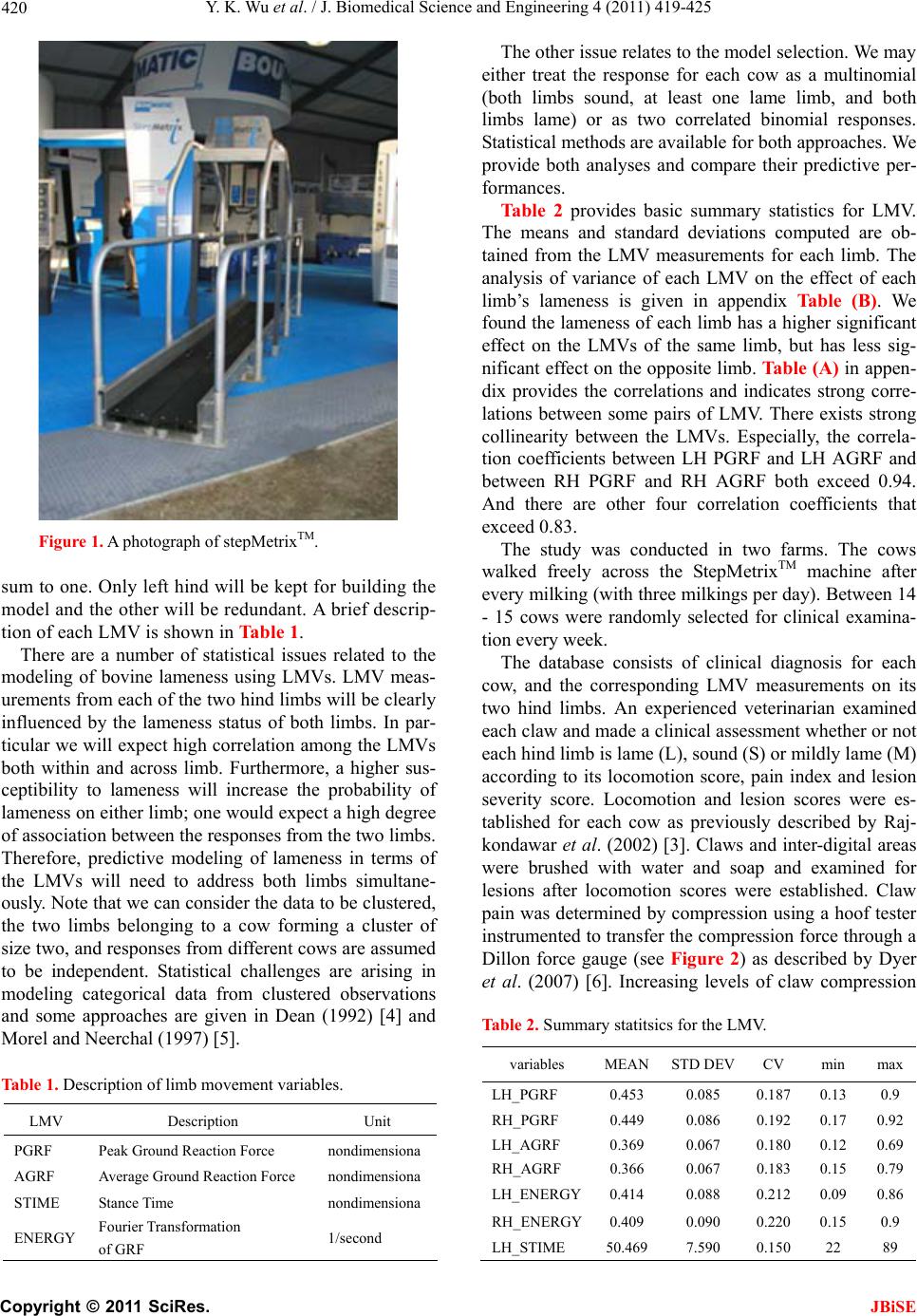

Y. K. Wu et al. / J. Biomedical Science and Engineering 4 (2011) 419-425 420
Figure 1. A photograph of stepMetrixTM.
sum to one. Only left hind will be kept for building the
model and the other will be redundant. A brief descrip-
tion of each LMV is shown in Table 1.
There are a number of statistical issues related to the
modeling of bovine lameness using LMVs. LMV meas-
urements from each of the two hind limbs will be clearly
influenced by the lameness status of both limbs. In par-
ticular we will expect high correlation among the LMVs
both within and across limb. Furthermore, a higher sus-
ceptibility to lameness will increase the probability of
lameness on either limb; one would expect a high degree
of association between the responses from the two limbs.
Therefore, predictive modeling of lameness in terms of
the LMVs will need to address both limbs simultane-
ously. Note that we can consider the data to be clustered,
the two limbs belonging to a cow forming a cluster of
size two, and responses from different cows are assumed
to be independent. Statistical challenges are arising in
modeling categorical data from clustered observations
and some approaches are given in Dean (1992) [4] and
Morel and Neerchal (1997) [5].
Table 1. Description of limb movement variables.
LMV Description Unit
PGRF Peak Ground Reaction Force nondimensiona
AGRF Average Ground Reaction Force nondimensiona
STIME Stance Time nondimensiona
ENERGY Fourier Transformation
of GRF 1/second
The other issue relates to the model selection. We may
either treat the response for each cow as a multinomial
(both limbs sound, at least one lame limb, and both
limbs lame) or as two correlated binomial responses.
Statistical methods are available for both approaches. We
provide both analyses and compare their predictive per-
formances.
Table 2 provides basic summary statistics for LMV.
The means and standard deviations computed are ob-
tained from the LMV measurements for each limb. The
analysis of variance of each LMV on the effect of each
limb’s lameness is given in appendix Table (B). We
found the lameness of each limb has a higher significant
effect on the LMVs of the same limb, but has less sig-
nificant effect on the opposite limb. Table (A) in appen-
dix provides the correlations and indicates strong corre-
lations between some pairs of LMV. There exists strong
collinearity between the LMVs. Especially, the correla-
tion coefficients between LH PGRF and LH AGRF and
between RH PGRF and RH AGRF both exceed 0.94.
And there are other four correlation coefficients that
exceed 0.83.
The study was conducted in two farms. The cows
walked freely across the StepMetrixTM machine after
every milking (with three milkings per day). Between 14
- 15 cows were randomly selected for clinical examina-
tion every week.
The database consists of clinical diagnosis for each
cow, and the corresponding LMV measurements on its
two hind limbs. An experienced veterinarian examined
each claw and made a clinical assessment whether or not
each hind limb is lame (L), sound (S) or mildly lame (M)
according to its locomotion score, pain index and lesion
severity score. Locomotion and lesion scores were es-
tablished for each cow as previously described by Raj-
kondawar et al. (2002) [3]. Claws and inter-digital areas
were brushed with water and soap and examined for
lesions after locomotion scores were established. Claw
pain was determined by compression using a hoof tester
instrumented to transfer the compression force through a
Dillon force gauge (see Figure 2) as described by Dyer
et al. (2007) [6]. Increasing levels of claw compression
Table 2. Summary statitsics for the LMV.
variables MEANSTD DEV CV min max
LH_PGRF 0.453 0.085 0.187 0.13 0.9
RH_PGRF 0.449 0.086 0.192 0.17 0.92
LH_AGRF 0.369 0.067 0.180 0.12 0.69
RH_AGRF 0.366 0.067 0.183 0.15 0.79
LH_ENERGY0.414 0.088 0.212 0.09 0.86
RH_ENERGY0.409 0.090 0.220 0.15 0.9
LH_STIME 50.4697.590 0.150 22 89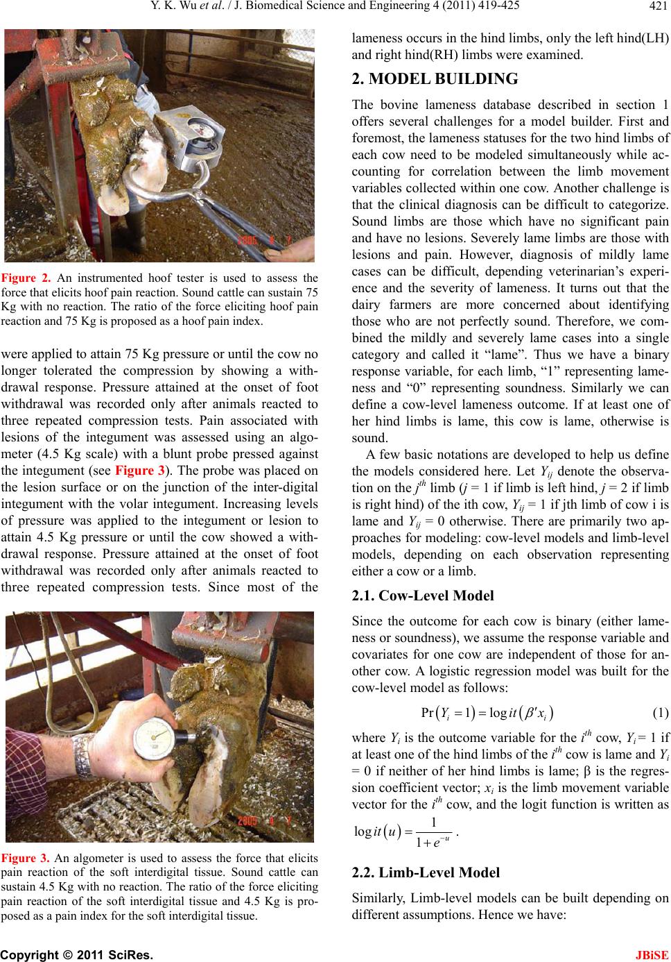

Y. K. Wu et al. / J. Biomedical Science and Engineering 4 (2011) 419-425 421
Figure 2. An instrumented hoof tester is used to assess the
force that elicits hoof pain reaction. Sound cattle can sustain 75
Kg with no reaction. The ratio of the force eliciting hoof pain
reaction and 75 Kg is proposed as a hoof pain index.
were applied to attain 75 Kg pressure or until the cow no
longer tolerated the compression by showing a with-
drawal response. Pressure attained at the onset of foot
withdrawal was recorded only after animals reacted to
three repeated compression tests. Pain associated with
lesions of the integument was assessed using an algo-
meter (4.5 Kg scale) with a blunt probe pressed against
the integument (see Figure 3). The probe was placed on
the lesion surface or on the junction of the inter-digital
integument with the volar integument. Increasing levels
of pressure was applied to the integument or lesion to
attain 4.5 Kg pressure or until the cow showed a with-
drawal response. Pressure attained at the onset of foot
withdrawal was recorded only after animals reacted to
three repeated compression tests. Since most of the
Figure 3. An algometer is used to assess the force that elicits
pain reaction of the soft interdigital tissue. Sound cattle can
sustain 4.5 Kg with no reaction. The ratio of the force eliciting
pain reaction of the soft interdigital tissue and 4.5 Kg is pro-
posed as a pain index for the soft interdigital tissue.
lameness occurs in the hind limbs, only the left hind(LH)
and right hind(RH) limbs were examined.
2. MODEL BUILDING
The bovine lameness database described in section 1
offers several challenges for a model builder. First and
foremost, the lameness statuses for the two hind limbs of
each cow need to be modeled simultaneously while ac-
counting for correlation between the limb movement
variables collected within one cow. Another challenge is
that the clinical diagnosis can be difficult to categorize.
Sound limbs are those which have no significant pain
and have no lesions. Severely lame limbs are those with
lesions and pain. However, diagnosis of mildly lame
cases can be difficult, depending veterinarian’s experi-
ence and the severity of lameness. It turns out that the
dairy farmers are more concerned about identifying
those who are not perfectly sound. Therefore, we com-
bined the mildly and severely lame cases into a single
category and called it “lame”. Thus we have a binary
response variable, for each limb, “1” representing lame-
ness and “0” representing soundness. Similarly we can
define a cow-level lameness outcome. If at least one of
her hind limbs is lame, this cow is lame, otherwise is
sound.
A few basic notations are developed to help us define
the models considered here. Let Yij denote the observa-
tion on the jth limb (j = 1 if limb is left hind, j = 2 if limb
is right hind) of the ith cow, Yij = 1 if jth limb of cow i is
lame and Yij = 0 otherwise. There are primarily two ap-
proaches for modeling: cow-level models and limb-level
models, depending on each observation representing
either a cow or a limb.
2.1. Cow-Level Model
Since the outcome for each cow is binary (either lame-
ness or soundness), we assume the response variable and
covariates for one cow are independent of those for an-
other cow. A logistic regression model was built for the
cow-level model as follows:


Pr1log
ii
Yitx 

 (1)
where Yi is the outcome variable for the ith cow, Yi = 1 if
at least one of the hind limbs of the ith cow is lame and Yi
= 0 if neither of her hind limbs is lame; β is the regres-
sion coefficient vector; xi is the limb movement variable
vector for the ith cow, and the logit function is written as

1
log 1u
it ue

.
2.2. Limb-Level Model
Similarly, Limb-level models can be built depending on
different assumptions. Hence we have:

Y. K. Wu et al. / J. Biomedical Science and Engineering 4 (2011) 419-425 422



12
345
12
345
Pr1 logij ij
ijij ij
ijj ijij
ij ij ij
Yitxx
xxx
 

 
 
(2)
where Yij is the outcome variable for the ith cow's jth limb.
j = 1 if it is left hind and j = 2 if it is right hind. In model
(2), we need to consider the following two possible con-
ditions: (a) there does not exist correlation between left
hind and right hind limbs within one cow, and (b) there
exists correlation between left hind and right hind limbs
within one cow. In the first case, ordinal logistic regres-
sion can be applied directly (SAS PROC LOGISTIC [7]).
In the second case, we need to consider within subject
correlation and GEE model can be applied (SAS PROC
GENMOD [7]).
If we neglect the difference between the left hind and
right hind limb-level models, assuming they have com-
mon intercept, we have:



12
345
12
345
Pr1 logij ij
ijij ij
ijij ij
ij ij ij
Yitxx
xxx
 

 
 
(3)
Similarly, we need to consider the existence of within
subject correlation in model (3). The selection between
the competent limb-level models can be obtained
through the likelihood ratio test for model (2) against
model (3).
3. LIKELIHOOD MODELS (Limb-level)
It is reasonable to assume that the responses of the two
limbs are correlated within each cow. Hence, overdis-
persion may exist. If we are allowed to assume the cor-
relation coefficient between the two hind limbs is the
same for each cow, in the likelihood framework, there
are two basic approaches to deal with overdispersion.
One is beta-binomial model [4], and the other is finite-
mixture model [5].
Here we demonstrate the likelihood function with fi-
nite-mixture approach. Let ρ2 be the correlation coeffi-
cient between the two limbs for each cow, and let piLH
and piRH be the probability of occurrence of lameness in
left hind and right hind limbs respectively for the ith cow.
The relationships of the lameness within each cow can
be summarized as follows in Table 3, where

2
11 11
,
iiLH iLHiRH iRH
iLH iRH
PPPPP
PP
  


10
211,
iiRHiLH iRH
iLH iLHiRH iRH
PP PP
PPPP 

 

01
211,
iiLHiLHiRH
iLHiLH iRHiRH
PPPP
PPPP 

 
Table 3. Probability distribution of occurrence of lameness
within ith cow.
LH
1 0 Marginal
1 Pi11 P
i10 P iRH
RH
0 Pi01 P
i00 1-PiRH
Marginal PiLH 1-PiLH 1
 ,11
1
2
01
iRHiRHiLHiLH
iRHiLHiRHiLHi
PPPP
PPPPP






and PiLH and PiRH are the probability of lameness in left
hind limb and right hind limb respectively for the ith cow.
The likelihood function can be expressed as:

n
ii
LL 1, where 00011011
00011011
iiii I
i
I
i
I
i
I
ii PPPPL ,
where IiLH is the indicator function of lameness status of
LH and RH limbs such that
Ii11=1 if both LH and RH limbs are lame,
=0 otherwise;
Ii10=1 if RH limb is lame and LH is sound,
=0 otherwise;
Ii01=1 if both RH limb is sound and LH is lame,
=0 otherwise;
Ii00=1 if both LH and RH limbs are sound,
=0 otherwise.
The log-likelihood function can be maximized (locally)
to find the maximal likelihood estimator (MLE) of the
parameters with appropriately chosen initial values (SAS
PROC NLP [8]). The estimated correlation coefficient is
ρ2 = 0.0861563, which indicates that the correlation be-
tween the two hind limbs is relatively small, and rea-
sonably neglectable. The beta-binomial model gives a
similar result.
4. NUMERICAL RESULTS
The modeling results with respect to sensitivity and spe-
cificity are summarized as follows in Tabl e s 4 , 5, 6 and
7. Here the lameness status indicator means the sound
category if its value is 0 and lame category if its value is
1, respectively.
5. CONCLUSION AND DISCUSSION
In this paper we discussed different approaches to model
bovine lameness with limb movement variables (LMVs),
generated by the StepMetrixTM system when a cow
walked through the machine. An experienced veterinar-
ian carefully examined and made a clinical assessment
of each hind claw of those randomly chosen cows in two
participating dairy farms. The lameness statuses assessed
by the veterinarian were used as “Gold Standard” to
evaluate the performance of several statistical models.

Y. K. Wu et al. / J. Biomedical Science and Engineering 4 (2011) 419-425 423
Table 4. Cow-level model.
Lameness status 0 (model) 1 (model) sum
0 (vet) 172 77 249
Specificity 69.08%
1 (vet) 32 75 107
Sensitivity 70.09%
Table 5. Cow-level model, without mildly lame cows in the
training data.
Lameness status 0 (model) 1 (model) sum
0 (vet) 117 42 159
Specificity 73.58%
1 (vet) 28 79 107
Sensitivity 73.83%
Table 6. Limb-level model.
Lameness status 0 (model) 1 (model) sum
0 (vet) 197 52 249
Specificity 79.12%
1 (vet) 21 86 107
Sensitivity 80.37%
Table 7. Limb-level model, without mildly lame cows in the
model.
Lameness status 0 (model) 1 (model) sum
0 (vet) 299 49 249
Specificity 80.32%
1 (vet) 17 90 107
Sensitivity 84.11%
We then compared the statistical model outputs with the
results given by the veterinarian. Ideally, we would like
to build a model that can detect lameness as soon as it
occurs in a cow, while avoiding false lameness flags.
From the above tables, the limb-level model, which ex-
cluded mildly-lame cow data from the model building,
demonstrated higher sensitivity and specificity than the
other limb-level model. The limb-level models, with or
without mildly-lame cows in the training data, overall
outperformed the cow-level models. Due to the existence
of noise in the LMVs, it is reasonable to exclude the
mildly-lame observations from the training data.
In the likelihood model with finite-mixture approach,
the estimated correlation coefficient is 2
ˆ

= 0:0861563,
which is small, indicating the correlation between lame-
ness status in the two hind limbs is negligible. Conse-
quently, the likelihood model is equivalent to the limb
level model if we neglect the correlation effect between
the two hind limbs.
In conclusion, after the evaluation of several statisti-
cal modeling approaches, the limb-level model with
mildly-lamb cow data excluded is superior to other
models. Additional analysis of the correlation of lame-
ness status between the two hind limbs showed very low
correlation between the two limbs. It is more probable
that the variation in lameness status of one hind limb
within each cow is more likely related to its own limb
movement variables rather than the lameness of the other
hind limb.
REFERENCES
[1] West, G.P. (1985) Black's veterinary dictionary. 15th
Rev Edition. A & C Black Publishers Ltd., London.
doi:10.3168/jds.2007-0496
[2] Thomsen, P.T., Munksgaard, L. and Tøgersen, F.A.
(2008) Evaluation of a lameness scoring system for dairy
cows. Journal of Dairy Science, 91, 119-126.
[3] Rajkondawar, P.G., Tasch, U., Lefcourt, A.M., Erez, B.,
Dyer, R. and Varner, M.A. (2002) A system for
identifying lameness in dairy cattle. ASABE Journal of
Applied Engineering in Agriculture, 18, 87-96.
[4] Dean, C.B. (1986) Testing for overdispersion in Poisson
and binomial regression models. Journal of American
Statistical Association, 87, 451-457.
doi:10.2307/2290276
[5] Morel, J.G. and Neerchal, N.K. (2007) Cluster binary
logistic regression using a finite mixture distribution with
application to teratology experiment. Statistics in Medi-
cine, 16, 2843-2853.
doi:10.1002/(SICI)1097-0258(19971230)16:24<2843::AI
D-SIM627>3.0.CO;2-F
[6] Dyer, R.M., Neerchal, N.K., Tasch, U., Wu, Y., Dyer, P.
and Rajkondawar P.G. (2007) Objective determination of
claw pain and its relationship to limb locomotion score in
dairy cattle. Journal of Dairy Science, 90, 4592-4602.
doi:10.1002/(SICI)10 97-0258(19 971230)1 6:24<28 43::AI
D-SIM627>3. 0.CO;2 -F
[7] Stokes, M.E., Davis, C.S. and Koch, G.G. (2009) Cate-
gorical data analysis using the SAS system. SAS Pub-
lishing, Cary.
[8] SAS Institute. (2007) SAS/OR 9.1.3 user's guide: Ma-
thematical programming. SAS Publishing, Cary.

Y. K. Wu et al. / J. Biomedical Science and Engineering 4 (2011) 419-425 424
Appendix
Table A. Correlations between the LMVs.
RH_PGRF LH_AGRF RH_AGRF LH_ENERGY RH_ENERGY LH_STIME
LH_PGRF 0.317 0.948 0.282 0.864 0.363 0.300
RH_PGRF 1 0.288 0.944 0.322 0.868 -0.382
LH_AGRF 1 0.287 0.843 0.348 0.296
RH_AGRF 1 0.306 0.838 -0.354
LH_ENERGY 1 0.385 0.190
RH_ENERGY 1 -0.263
ANOVA tables of LMVs on Lameness status:
Table B1. ANOVA Table of LHLAMESCORE on LH_PGRF.
Source DF Sum of Squares Mean Square F ValuePr > F
Model 1 0.352144 0.352144 58.38 <.0001
Error 354 2.135168 0.006032
Total 355 2.487311
Table B2. ANOVA Table of LHLAMESCORE on LH_AGRF.
Source DF Sum of Squares Mean Square F ValuePr > F
model 1 0.267368 0.267368 72.84 <.0001
error 354 1.29931 0.00367
total 355 1.566677
Table B3. ANOVA Table of LHLAMESCORE on LH_STIME.
Source DF Sum of Squares Mean Square F Value Pr > F
Model 1 2873 2873 54.88 <.0001
Error 354 18532.1 52.35057
Total 355 21405.1
Table B4. ANOVA Table of LHLAMESCORE on
LH_ENERGY.
Source DF Sum of Squares Mean Square F ValuePr > F
model 1 0.317513 0.317513 43.75<.0001
error 354 2.569063 0.007257
total 355 2.886576
Table B5. ANOVA Table of RHLAMESCORE on LH_AGRF.
Source DF Sum of Squares Mean Square F ValuePr > F
model 1 0.005813 0.005813 1.32 0.2517
error 354 1.560864 0.004409
total 355 1.566677
Table B6. ANOVA Table of RHLAMESCORE on LH_PGRF.
SourceDFSum of SquaresMean Square F ValuePr > F
Model 1 0.005795 0.005795 0.83 0.3638
Error 3542.481516 0.00701
Total 3552.487311
Table B7. ANOVA Table of RHLAMESCORE on LH_PGRF.
Source DF Sum of SquaresMean Square F ValuePr > F
Model 1 0.001595 0.001595 0.2 0.6585
Error 3542.884981 0.00815
Total 355 2.886576
Table B8. ANOVA Table of RHLAMESCORE on RH_PGRF.
Source DFSum of Squares Mean Square F ValuePr > F
Model 1 0.029742 0.029742 4.16 0.042
Error 3542.528093 0.007142
Total 3552.557835
Table B9. ANOVA Table of LHLAMESCORE on RH_AGRF.
Source DF Sum of Squares Mean Square F ValuePr > F
Model 1 0.017994 0.017994 4.41 0.0364
Error 3541.443479 0.004078
Total 3551.461473
Table B10. ANOVA Table of LHLAMESCORE on
RH_ENERGY.
SourceDFSum of SquaresMean Square F ValuePr>F
Model 10.00409 0.00409 0.52 0.4734
Error 3542.810259 0.007939
Total 3552.814349

Y. K. Wu et al. / J. Biomedical Science and Engineering 4 (2011) 419-425 245
Table B11. ANOVA Table of RHLAMESCORE on
RH_AGRF.
Source DF Sum of Squares Mean Square F ValuePr>F
Model 1 0.275075 0.275075 82.08 <.0001
Error 354 1.186398 0.003351
Total 355 1.461473
Table B12. ANOVA Table of RHLAMESCORE on
RH_PGRF.
Source DF Sum of Squares Mean Square F ValuePr>F
Model 1 0.384894 0.384894 62.7 <.0001
Error 354 2.17294 0.006138
Total 355 2.557835
Table B13. ANOVA Table of RHLAMESCORE on
RH_STIME.
Source DFSum of SquaresMean Square F ValuePr>F
Model 1 3544.426 3544.426 70.27<.0001
Error 35417855.09 50.4381
Total 35521399.51
Table B14. ANOVA Table of RHLAMESCORE on
RH_PGRF.
SourceDFSum of SquaresMean Square F Value Pr>F
Model 1 0.264919 0.264919 36.79 <.0001
Error 3542.549431 0.007202
Total 3552.814349