 American Journal of Computational Mathematics, 2011, 1, 83-103 doi:10.4236/ajcm.2011.12009 Published Online June 2011 (http://www.scirp.org/journal/ajcm) Copyright © 2011 SciRes. AJCM 83 Methods of Approximation in hpk Framework for ODEs in Time Resulting from Decoupling of Space and Time in IVPs K. S. Surana1*, L. Euler1, J. N. Reddy2, A. Romkes1 1Mechanical Engineering, Department, University of Kansas, Lawrence, USA 2Mechanical Engineering D e pa rtment, Texas A&M University, College Station, USA E-mail: kssurana@ku.edu, jnreddy@tamu.edu Received March 28, 2011; revised May 26, 2011; accepted Jun e 3, 2011 Abstract The present study considers mathematical classification of the time differential operators and then applies methods of approximation in time such as Galerkin method (GM ), Galerkin method with weak form (/GMWF ), Petrov-Galerkin method (PGM), weighted residual method (WRY ), and least squares method or process (LSM or LSP ) to construct finite element approximations in time. A correspondence is estab- lished between these integral forms and the elements of the calculus of variations: 1) to determine which methods of approximation yield unconditionally stable (variationally consistent integral forms, VC ) com- putational processes for which types of operators and, 2) to establish which integral forms do not yield un- conditionally stable computations (variationally inconsistent integral forms, VIC). It is shown that varia- tionally consistent time integral forms in hpk framework yield computational processes for ODEs in time that are unconditionally stable, provide a mechanism of higher order global differentiability approxima- tions as well as higher degree local approximations in time, provide control over approximation error when used as a time marching process and can indeed yield time accurate solutions of the evolution. Numerical studies are presented using standard model problems from the literature and the results are compared with Wilson’s method as well as Newmark method to demonstrate highly meritorious features of the pro- posed methodology. Keywords: Finite Element Approximations, Numerical Studies, Time Approximation, Variationally Consistent Integral Forms 1. Introduction, Literature Review and Scope of Work The quest for better, reliable, stable, accurate and effi- cient methods of approximation for obtaining numerical solutions of the ordinary differential equations (ODEs ) in time resulting from either decoupling of space and time or using a lumped parameter approximation in spa- tial coordinates in initial value problems has been a sub- ject of writing in the numerical and computational me- thods area for over a century. Thus, the published works are voluminous. In this section we provide a summary of historical perspective of the origins of various methods, discuss more recent advances in the various approaches, discuss their merits and shortcomings with the objective of ultimately narrowing down to a single methodology that provides us an infrastructure to treat all ODEs in time in a consistent but rigorous manner without any regard to specific applications or their origin. 1.1. Space-Time Decoupling in IVPs We make a few remarks regarding a strategy for space- time decoupling in initial value problems ( VPs ) that lead to ODEs in time. This is helpful in gaining a bet- ter understanding regarding the origin of the ODEs . The VPs are generally a system of partial differential equations in dependent variables, spatial coordinates and time. Thus, these naturally contain spatial as well as time derivatives of the dependent variables. In decoupling of  K. S. SURANA ET AL. Copyright © 2011 SciRes. AJCM 84 space and time, the spatial derivatives are converted into algebraic expressions, thereby reducing the original par- tial differential equations (PDEs ) to a system of ODEs in time. For this purpose we can use finite difference, finite volume or finite element method in spatial coordi- nates. In a finite difference method one discretizes the spatial domain into a finite number of points. The spatial derivatives are approximated using Taylor series expan- sions of various orders of truncation errors to obtain al- gebraic expressions or the finite difference approxima- tions of the spatial derivatives. One then considers the PDEs at each point of the discretization and substitutes the finite difference expressions for the spatial deriva- tives. The outcome of this process is that spatial deriva- tives are replaced by dependent variable values (and/or their derivatives) at the points of the discretization and the time derivatives assume values at the points of the discretization and thus we obtain a system of ODEs in time. In principle, the finite volume method of decoup- ling space and time is similar. In the finite element method of decoupling space and time, one constructs a spatial discretization of the spatial domain using finite elements. We can construct an integral form over the discretized spatial domain based on the fundamental lemma [1-5]. The time derivatives for this purpose are treated as constants. One constructs an approximation over the discretized domain and thereby an approxima- tion over each spatial element of the discretization. This approximation, when substituted in the integral form, replaces the spatial derivatives with algebraic expres- sions and what remains is a system of ODEs in time. In the following, we present some details of the finite element method of decoupling space and time. Let (, )(, )0, (, )(0, )(0, ) xtx t Axtfxt xt L (1.1) be an initial value problem with some boundary condi- tions (BCs ) and some initial conditions ( Cs ). Let Te x e be a finite element discretization of . Let (, ) h t be an approximation of (, ) t over T Then based on the fundamental lemma [1-5] of the calculus of variations, ((, )(, ), )0 T x h Axt fxtv (1.2) in which ()vvx is the test function. v is zero where is specified, thus h v is admissible. We can write (1.2) over () T x as, ((, )(, ), )0 e x e h e Axtfxtv (1.3) where (, ) e h t is the local approximation of (, ) t over e . Consider ((, ), ) e x e h xtf v over an ele ment e with domain e . At this point if the operator A has even order derivatives with respect to spatial coor- dinates, then one could use integration by parts to trans- fer half of the differentiation from e h to v (Galerkin method with weak form in space) and then the resulting expression could be arranged as (, )(, )(, )() ee xx eee e hh fvBv fvlv (1.4) in which () e lv is the concomitant. It contains the boundary terms (secondary variables) due to integration by parts. Let the local approximation (, ) e h t be given by 1 (, )()() n ee hii i tNxt (1.5) Consider Galerkin method with weak form, () e hj vNx , 1, 2,,jn (1.6) Substituting (1.5) and (1.6) into (1.4) we can write (assuming that operator has first and second order derivatives of in time as well as the function ) 123 (, )[][][] () (, ); 1,, e x eeee ee ee h ee ej BvCC C lv P FfNjn (1.7) e is a vector of secondary variables. Thus, 123 (, ) ([ ][ ][ ]) e x e h ee ee eeee Afv CCC PF (1.8) Substituting from (1.7) into (1.4) we have, 123 () ([ ][ ][ ]) 0 e x e h e ee ee ee e ee ee Af CCC PF (1.9) or 123 [][ ][]CCC PF (1.10) in which 112 233 [][], [][], [][], , eeee eee ee ee CCCCCC PPFF (1.11) and , , eee eee (1.12) (1.10) are a system of ODEs in time. A solution of  K. S. SURANA ET AL. Copyright © 2011 SciRes. AJCM 85 these in time would yield and thereby e for each element of the spatial discretization and hence, the approximation (, ) e h t for an element defined by (1.5) completely defines the evolution. This paper considers the finite element method of ap- proximation for a system of ODEs in time (like (1.10)) resulting from space-time decoupling in VPs . 1.2. Literature Review The published work addressing the methods of approxi- mation for ODEs in time is heavily dominated by finite difference methods or methods like finite difference methods that originate from the use of Taylor series ex- pansions at discrete points in the time domain to ap- proximate time derivatives in the ODEs by algebraic expressions containing function values and/or their de- rivatives at the discrete points in the time domain [0, ] x . In the following we discuss some of the commonly used approaches. Reference [6] presents various methods of approxima- tion (primarily based on the Taylor series expansions) for ODEs in time. In reference [7] the authors present an account of the various methodologies for approximating solutions of ODEs in time. These include details for first order symmetric systems, second order symmetric systems, as well as nonlinear symmetric and nonsym- metric systems of ODEs . One step algorithms, linear multistep ()LMS algorithms, Houbolt method, -me- thod and partitioning methods are considered as methods of approximation. Some discussion on convergence and stability is also presented. Perhaps the most significant work amongst the earlier works is due to Newmark [8] based on the assumption of linear acceleration in a time interval. Another parallel work by Wilson [9], Wilson’s method, is also as significant. This is also based on the assumption of linear acceleration in a time interval. These two works were strictly aimed at ODEs from decoupling space and time in structural dynamics (sec- ond order ODEs in time). In the Newmark method the equilibrium is considered at time tt at which the evolution state is not known. In Wilson’s method the linear acceleration assumption is extended to the time interval [, ]tt t , 1 . The equilibrium is consid- ered at time tt but the evolution is computed at time tt . The value of is determined from the stability analysis of the method. It is shown that for 1.37 (generally chosen 1.4), the Wilson’s method is unconditionally stable. Many works using the two approaches have appeared in the literature in which accuracy (amplitude decay, base elongation and phase shift of known and specified waves) and applications of these methods have been discussed. A modification of Newmark method referred to as alpha modification is presented in reference [10]. The additional parameter alpha is introduced to achieve simultaneous second order accuracy, unconditional sta- bility and positive artificial damping. A family of “one step unconditionally stable integration schemes with im- proved numerical dissipation” is presented in reference [11]. The “generalized -method in structural dynam- ics” is presented in reference [12] with “user controlled numerical dissipation”. Extensions of LMS methods to L-stable optimal integration methods with 0u-0v overshoot properties in structural dynamics are given in reference [13]. This approach leads to level-symmetric (LS) integration methods. The LS methods are cre- ated as symmetric variants of extended three level LMS methods (3L-LMS ) with direct use of dynamic equa- tions to obtain algorithmically simple integration schemes that have maximum damping of high frequency modes and thereby without overshoots. The analysis of generalized -method for non-linear dynamic problems is presented in reference [14]. It is shown that general- ized α-methods have stability in the energy sense and guaranteed energy annihilation. But, these methods ex- hibit overshoots and heavy energy oscillations in inter- mediate frequency ranges. The energy-conserving and decaying algorithms in structural dynamics based on -method are considered in reference [15]. In a series of papers [16-22], exhaustive developments and details are presented related to time integration of ODEs . A detailed discussion of various aspects, their merits and shortcomings are not relevant in view of the ap- proach presented in this paper and is also too voluminous to be included here. However, we do remark that various approaches in these papers utilize weighted residual concepts, Taylor series expansions, Taylor series expan- sion in time and /GMWF and consider single step and multistep algorithms. Stability, accuracy and other fea- tures of the various proposed schemes are presented in- cluding numerical studies for model problems. 1.3. Scope of Present Work and Methodology We want to take a very pragmatic view i.e., we pose a question “What is our objective?” The answer of course is, we want to consider a method of approximation for ODEs in time that has the following features. 1) The methodology must be equally applicable to all ODEs , i.e., must be independent of the nature of the time operator. 2) The method must be unconditionally stable regard- less of the choice of integration time step. 3) The method must be time marching so that the computations of the evolution can be done for an incre-  K. S. SURANA ET AL. Copyright © 2011 SciRes. AJCM 86 ment of time. This is essential for computational effi- ciency in applications requiring the evolution for long periods of time as well as in applications in which a large number of ODEs are involved. 4) The method must permit higher degree approxima- tion of the solution in time for an increment of time. 5) To ensure desired global differentiability of the ap- proximation over t we must ensure that the time ap- proximations of higher degree for each increment of time are such that their union indeed yields desired global differentiability of the approximation in time. For exam- ple if an ODE in time contains up to second order de- rivatives of the dependent variable and if the theoretical solution is analytic, then the approximation of this solu- tion over t must at least be of class 2() t C. 6) There must be a measure (and not estimation) of approximation errors in the computed solution regardless of whether we have a theoretical solution of the ()ODE s or not. This feature is essential due to the fact that most problems of practical interest do not permit determination of a theoretical solution, yet it is essential to know the approximation errors in the computed solu- tion to determine if the computed solution satisfies the desired requirements of accuracy. 7) There must be a mechanism to reduce the approxi- mation errors to whatever desired level so that a desired accuracy is achievable in the computed solution. 8) The methodology must permit time accurate evolu- tions. This aspect becomes intrinsic in the approach if features 6) and 7) are present. The features described above are indeed intrinsically present in the mathematical and computational infra- structure presented in this paper for ODEs in time. Section 2 describes the mathematical details of the for- mulation, approximations and approximation spaces as well as details of the computational infrastructure.The requirements 1) - 8) are described in the paragraph above are all addressed in Section 2. It is shown that the finite element discretization in time in which the local ap- proximations in time are in hpk framework permitting global differentiability of the approximation of order (1k) in time when used with integral forms that are variationally consistent provides a mathematical and computational infrastructure for ODEs in time with all of the desired attributes. Numerical studies are presented in Section 3 for commonly used model problems and the numerical results from the present work are compared with Newmark and Wilson’s method. 2. Finite Element Approximation of ODEs in Time For presenting the mathematical details and formulations it suffices to consider a single ODE in time. 0AdF 0 (0, )(, ) t tt (2.1) with some initial conditions. is a differential opera- tor in time or time differential operator. 2.1. Mathematical Classification of Time Differential Operators If (2.1) represents totality of all ODEs regardless of the application, then we must classify time differential op- erators mathematically so that we could consider development of the methods of approximation for this classification with mathematical rigor. The simplest possible classification of course is where the operator is either linear or non-linear. Definition. 1: The time operator is linear if u , A vD , the domain of definition of the operator and , , the following holds () u vAuAv (2.2) Definition. 2: If the time operator is not linear then it is non-linear. This classification can be made more restrictive by considering symmetry (or lack of it) of . Definition. 3: The time operator is symmetric if it is linear and if u , A vD , the domain of the fol- lowing holds (, )(, ) tt uv uAv (2.3) We note that (2.3) requires differential operator in that we transfer all of the time or time differential time dif- ferentiation from u to v (left side of (2.3)) using in- tegration by parts. In doing so, we obtain the following in general, (, )(, ), tt uv uAv Auv (2.4) is called the adjoint of and , uv is called the concomitant which results as a consequence of inte- gration by parts. Thus, based on the definition of sym- metry in (2.3), if is symmetric, then A (2.5) , 0Auv (2.6) That is, the adjoint of the time operator must be the same as the time operator and the concomitant must be zero. When the operator has even order de- rivatives in time then we could show that (2.5) holds. Thus, there are time differential oeprators for which (2.5) is possible. (2.6) contains boundary terms and hence it can be expanded. 0 , , , t uv AuvAuv (2.7) In (2.7), 0 t and are the boundaries of the time domain at 0 tt (initial conditions) and at t an  K. S. SURANA ET AL. Copyright © 2011 SciRes. AJCM 87 open boundary. Let us assume that based on Cs it is possible to show that 0 , 0 t Auv , then for symmetry of we must show that , 0Au v so that (2.6) will hold. is an open boundary where neither the function nor its time derivatives are known, hence it is not possible to show that , uv is zero. Since an open boundary at t exists in case of all ODEs regardless of whether is linear or non-linear, for time differential operators , (2.6) can not be satisfied, hence the time differential operators can not be symmet- ric. This leads to the following two categories of mathe- matical classification for all time differential operators. Definition. 4: If a time differential operator is linear then it is non-self adjoint Definition. 5: If a time differential operator is not linear then it is obviously non-linear 2.2. Methods of Approximation in Time (Based on Time Integral Forms) Before we consider finite element method of approxima- tion it is perhaps more prudent to consider classical methods of approximation in time (these consider t without discretization) for the two classes of operators to determine which methods of approximation are worthy of consideration in the finite element processes in time. We group the methods of approximation (based on integral form in time) in two categories: 1) those based on fundamental lemma [1-5] 2) those based on minimization of the residual func- tional [23,24] 2.2.1. Methods Based on Fundamental Lemma The methods such as GM , PGM , WRM and / GMWF in time are the methods in this category. In all these methods we begin by using fundamental lemma [1-5] over t . If n d is the approximation of d over t , then (, )0 t n AdFv (2.8) in which v is test function. 0v on if 0 dd (known) on . In GM and /GMWF we consider n v . In PGM () n vt and in WRM also () n vwt . We can write (2.8) as (, )(, ) tt n dv Fv or (, )() n Bd vlv (2.9) In / GMWF we also begin with (2.8) i.e. , (, )(, ) tt n dv Fv (2.10) but transfer some differentiation from n d to v to ob- tain a weak form in time, (, )()(, )() t n BdvlvF vlv (2.11) Thus all these methods of approximation in time yield a time integral form ((2.9) or (2.11)). () n dt is ex- pressed as 0 1 ()()( )() n nii i dt NtNxtc (2.12) in which () i Nt are basis functions. Obviously () n dt must satisfy all Cs of the ODE . When (2.12) and ();1, 2,, or () or ();1, 2,, nj jj vNtjn vtvwtjn (2.13) are substituted in (2.9) or (2.11), we obtain a system of linear or non-linear algebraic equations in i c from which we can determine i c. Remarks 1) These methods of approximation result in an inte- gral form that is converted to an algebraic system upon substituting the approximation. The algebraic system is used to determine the unknowns i c. Thus in these methods we have a “necessary condition” only. 2) Existence and uniqueness of the solution n d or the coefficients i c is never addressed, hence must be con- sidered for each application. 3) This situation can be corrected by establishing a correspondence between the integral forms (necessary conditions) and the calculus of variations. 2.2.2. Variationally Consistent and Variationally Inconsistent Time Integral Forms Consider extremum of a functional () n d i.e., assume that there exists a functionan () n d and we wish to determine its extremum. Then, 1) Existence of () n d is generally by construction. 2) Necessary condition: If () n d is differentiable in n d and if the deriva- tives of all orders are continuous then, based on the theorems of calculus of variations () n d is unique and ()0 n Id is a necessary condition for the existence of the extremum of () n d. 3) The sufficient condition or extremum principle is given by 2 0minimum of () ()0saddle point of () 0maximum of () n nn n d dId d (2.14) When we have a unique extremum principle, then we can show that a n d obtained from ()0 n Id also satisfies the Euler’s equation, a differential equation that can be obtained from ()0 n Id . Thus, we have a cor-  K. S. SURANA ET AL. Copyright © 2011 SciRes. AJCM 88 respondence between the solutions of differential equa- tions and the elements of the calculus of variations deal- ing with extremums of functionals. We proceed as fol- lows. Let 0Ad F be the ODE in time. Then there must exist a functional () n d such that ()0 n Id gives the integral form (from any of the chosen methods of approximation) and 2() n d yields a unique extremum principle and the Euler’s equation from ()0 n Id is the ODE , then a n d that yields a unique extremum of () n d is also a unique solution of 0Ad F . Definition. 6: Variationally consistent (VC ) integral forms. A time integral form resulting from a method of approximation is termed VC if there exists a functional () n d such that () 0 n Id gives the integral form and 2() n d yields a unique extremum principle. Definition. 7: Variationally inconsistent (VIC) time integral forms. A time integral form resulting from a method of approximation is termed VIC if it is in vio- lation of one or more elements of the calculus of varia- tions. It is sufficient to show the following. Let there exist a functional () n d such that ()0 n Id gives the desired integral form. Then 2() n d i.e. the first variation of the integral form must yield a unique extre- mum principle. It is straight forward to show (see [24]) that the time integral forms resulting from GM , PGM , WRM and / GMWF are all variationally inconsistent. Variation- ally consistent integral forms yield algebraic systems in which the coefficient matrices are symmetric and posi- tive definite and uniqueness of the solution n d is en- sured. VIC integral forms, on the other hand, yield non-symmetric coefficient matrices that are not always ensured to be positive definite. See references [23,24] for more details. Thus, GM ,PGM ,WRM and /GMWF in time are not worthy of consideration for finite element processes in time as a general computational methodol- ogy for ODEs in time as these do not ensure uncondi- tionally stable computations due to VIC integral forms in time. 2.2.3. Methods of Approximation Based on Minimiza- tion of Residual Functional In this category of methods we consider least squares method or process (LSM or LSP ) in time based on residual functional. Let n EAd F t t (2.15) define residual E over the time domain t . 1) Existence of a functional () n d (residual func- tional) is by construction. ()(, ) t n dEE (2.16) () n d is a convex function of E, regardless of the mathematical classification of 2) Necessary condition ()2(, )0 t n IdE E (2.17) or (, )()0 tn EE gd (2.18) 3) Sufficient condition or extremum principle 22 ()2(, )2(, ) tt n dEEEE (2.19) In the following we consider the two categories of the mathematical classification of i.e., when is non-self adjoint and when is non-linear, and deter- mine variational consistency or variational inconsistency of the time integral form given by (2.18). Case (a): When is non-self adjoint In this case the operator is linear, hence 20E and the extremum principle 2 given by 2()2(, )0 t nn dEEd (2.20) Thus, we have a unique extremum principle. (2.20) im- plies that a n d obtained from (2.18) minimizes () n d in (2.16) Case (b): When is non-linear In this case 2E is not zero. We note that ()0 n Id yields ()(, )0 t n gdEE (2.21) in which () n d is a non-linear function of n d. Thus, we must find n d iteratively such that (2.21) is satisfied. We choose Newton’s linear method. Let 0 n d be an as- sumed or guess of n d then, 0 ()0 n gd (2.22) Let n d be a change or a correction to 0 n d such that 0 ()0 nn gd d (2.23) Expanding 0 () nn dd in Taylor series about 0 n d and retaining only up to linear terms in n d. 0 00 ()() 0 n nn nn d n g gddgdd d (2.24) From (2.24), we can solve for n d. 0 1 0 () n nn d n g dgd d (2.25) We note that 22 (, ) 1 (, )(, )() 2 t tt n n ggEE d EEE EId (2.26) If n d is positive definite in (2.25), then we are  K. S. SURANA ET AL. Copyright © 2011 SciRes. AJCM 89 ensured a unique solution n d Based on (2.26), this is possible if we approximate 2() n d by [25-31] 2()2(, )0, a unique extremum principle t n IdE E (2.27) Rationale for the approximation in (2.27) has been discussed by Surana et.al. [23-27,32,33]. Thus, with (2.27) the LSP in time for ODEs in time in which the differential operator is non-linear is variationally consistent. Once we find a n d using (2.25), it is helpful to consider the following for obtaining an updated solution n d 0 nn n dd d (2.28) in which is a scalar generally between 0 and 2 and assumes the largest value between 0 and 2 for which 0 () () nn dId holds. This is referred to as line search. The entire process of solving for n d that satisfies ()0 n gd is called Newton’s linear method with line search. 2.2.4. Remarks on Methods of Approximation in Time Based on Integral Forms in Time 1) The determination of variational consistency or variational inconsistency of an integral form in time al- lows us to determine unconditional stability of the re- sulting computations which helps in deciding which in- tegral forms in time are worthy of consideration for the development of finite element method in time for the ODEs in time. 2) The time integral forms resulting from GM , PGM , WRM and /GMWF in time are all varia- tionally inconsistent regardless of whether the time op- erator is non-self adjoint or non-linear. 3) The time integral form resulting from the LSP in time based on residual functional is variationally consis- tent when the time differential operator is non-self adjoint. 4) The time integral form resulting from the LSP in time based on residual functional for non-linear time operators is also variationally consistent provided a) n d in ()0 n gd is determined using Newton’s linear method, and b) the second variation of the residual func- tional is approximated by 2()2(, ) t n dEE 5) Based on (1-4), it is obvious to conclude that only LSP in time based on the residual functional is merito- rious of consideration as a general numerical solution methodology for developing finite element processes in time for ODEs in time. This would be applicable to the totality of all ODEs as it yields VC integral forms for both non-self adjoint and non-linear operators in time. 2.3. Finite Element Processes in Time Based on Minimization of a Residual Functional: Least Squares Finite Element Process In this section we present details of finite element proc- esses in time based on least squares method using the residual functional. Consider an ODE in time, 0Ad F 0 (0, )(, ) t tt (2.29) with some initial conditions. Let () Te tt e be a time discretization of t in which e t is a typical element e (for example a three node p-version ele- ment). Let () h dt be the approximation of () T t dt and () ee ht dt t be the local approximation of ()dt for an element e of the discretization such that () () e hh e dt dt (2.30) We consider the residual functional E over the dis- cretization () T t . n EAd F () T t t (2.31) 1) Least squares functional over () T t () ()(, )(, )() Te tt ee ee nh ee dEEEEId (2.32) 2) Necessary condition ()()(, ) 2(, )2(, ) 2{()}2()0 e t ee tt eeee hh ee ee ee ee ee hh e IdI dEE EE EE gd gd (2.33) or ()()0 ee hh e gdgd (2.34) We find a h d that satisfies (2.34), i.e., (2.34) is used to solve for h d and thereby e h d. 3) Sufficient condition or extremum principle: 2() h d gives the the extremum principle. 2 2 () (())(()) 2((, )) 2(, )2(, ) e t ee tt ee hh h e ee e eee e ee IdIdI d EE EEE E (2.35) Case (a): When is non-self adjoint In this case, is linear, hence, () ee h EAdFAv e t t (2.36)  K. S. SURANA ET AL. Copyright © 2011 SciRes. AJCM 90 2()()0 ee EEAv (2.37) Hence, the necessary condition becomes ()(, ) e t ee h ee gdE E (, )0 e t e h e AdFAv (2.38) and the extremum principle, 2()2(, ) 2(, )0 e t e t ee he e IdE E Av Av (2.39) Hence, a unique extremum principle. Consider the lo- cal approximation () e h dt. 1 ()(); ()(); 1, 2,, n eee hiinj i dtNtd vdtNt jn (2.40) Consider (, ) e t e h dFAv in (2.38) for an element e. (, )(, ) ee tt ee hh Ad FAvAvAd F (2.41) (()) j vANt ; 1, 2,,jn (2.42) or {} e vE (2.43) 1 (()){}{ } n eeete hii i AdANdE (2.44) Substituting from (2.43) and (2.44) into (2.41) and noting that, (, )(, )(, ) eee ttt ee hh v AdFAv AdFAv (2.45) or (, )({}, {}{}) ({}, {}){}(, {}) ee tt ee tt eeete h eete e Av AdFEE EE FE (2.46) or (, )[]{}{} eeee h vAdFKF (2.47) in which e ij of [] e and e i of {} e in are given by ((()), (())) , 1, 2,, (, (())) e t e t e ij ij e ii KANtANtij n FFANt (2.48) ee ij ji K, i.e., [] e is symmetric, a consequence of VC integral forms in time resulting from LSP in time based on the residual. Substituting from (2.47) into (2.38), we obtain the following for the discretization () T t . ()([]{} {})0 ee e he gd KF (2.49) or []{}{} F (2.50) where [][], {}{ } and {}{} ee ee e e KKFF (2.51) Case (b): When is non-linear In this case is a function of d, hence ()()() (), in which v= hhh hh EAdFAd Ad vAd d (2.52) and ()()() (), in which = eee e hhh ee hh EAdFAdAd vAd vd (2.53) ()(, ) (, ())0 e t e t ee he ee hh e gdE E AdFAvA d (2.54) Using the local approximation (2.40) and noting that {}{ } e e , {} e being nodal degrees of freedom e i d for an element ‘e’, we have, (){({})}0 h gd g (2.55) That is, is a non-linear function of nodal degrees of freedom {} . Using, Newton’s linear method (as described earlier) we obtain, 0 1 0 {} () {} {({})} () gg (2.56) {} is the incremental change in the assumed solu- tion 0 {} . But, 2 2 () () {} 1 {} {} 2 (, )(, ) TT tt ggI EEEE (2.57) Thus 0 210 1 {}[ ]{({})} 2Ig (2.58) For a unique {} , the coefficient matrix in (2.58) must be positive definite. This is possible if we approximate 2 by, 2 () 2(, )0 T t IEE (2.59) which yields a unique extremum principle and we have, 0 10 (){} {}[(, )]{({})} T t EE g (2.60) An improved solution is obtained using 0 {} {}{} (2.61) Details of line search involving remain the same as presented earlier. We note the coefficient matrix in  K. S. SURANA ET AL. Copyright © 2011 SciRes. AJCM 91 (2.60) is () (, )(, ) Te tt ee e EEE E (2.62) Recalling ()() ee h EAvAd (2.63) and ({})({})(, )e t eeee ee gg EE (2.64) thus the right side of (2.60) is completely defined to de- termine {} . The convergence of the Newton’s linear method is checked based on i g i.e., the absolute value of each component of {} must be below a threshold value representing a numerically computed zero. 2.4. Approximation Spaces We consider local approximation functions () i Nt in an approximation space h V; a subspace of , () kp e t H space, i.e. , ()( ) kp e ih t Nt VH (2.65) and since 1 n ee hii i dNd in which e i d are constants, we ensure that e hh dV (2.66) k is the order of the approximation space defining global differentiability of () () e hh e dt dt of order (1k) and p is the degree of local approximation of () e h dt. The minimum value of k for which the integrals in the LSP in time are Rieman defines the minimally conforming space. For value k one lower than mini- mally conforming, the integrals become Lebesgue. These approximation spaces permit change in h, the element length in time, control over p, the degree of local ap- proximation and k, the order of the space, hence re- ferred to as hpk framework [23-27,32,33]. 2.5. Benefits and Meritorious Features of the Proposed LS Finite Element Formulation for ODEs in Time in hpk Framework 1) Due to the mathematical classification of all time operators into non-self adjoint and non-linear categories, the task of the development of the methods of approxi- mation for ODEs in time is reduced to these two cate- gories that address the totality of all time operators. 2) The investigation of the VC of the time integral forms resulting from various methods of approximation reveals that only the time integral forms resulting from the LSP in time based on the residual are variationally consistent for both classes of differential operators. The finite element processes proposed here are based on LSP in time, hence they yield unconditionally stable computations for all choices of computational and physical parameters for both categories of differential operators in time. 3) The method can be obviously made time marching. One considers only one element in time and time marches in sequel to compute the entire evolution. This results in efficiency of computations. 4) The degree of local approximation p permits de- sired polynomial for local approximation over an ele- ment in time. The local approximations can also be hier- archical. This adds additional efficiency in the computa- tional processes for linear operators if p-levels are in- creased progressively. 5) Since () i Nt and hence , ()( ) ekpe hht dt VH , the time approximation () () e hh e dt dt can be ensured to be of any desired global differentiability in time. This helps in maintaining the integrals in the computational process in the Riemann sense. Higher values of k than minimally conforming permit us to incorporate higher order global differentiability of the theoretical solution in the computational process if so desired. 6) In the LSP in time, we note that a h d obtained from 2() 0 h Id minimizes () h d due to the fact that 2()0 h Id . But () h d is a convex function of E, hence its minimum is zero. Thus, when h dd, () 0 h Id which implies that 0() T t Et in the pointwise sense if the integrals in the entire process are Riemann. Since the theoretical value of () h d i.e., () d is zero, () h d is a measure of error in the solu- tion over () T t and likewise () ee h d are measures of error in each element (if one uses a mesh in time). 7) In the approach presented here, we choose an ele- ment in time (thereby choosing h) and a minimally conforming k and conduct a p-convergence study to ensure that () h d is as closeto zero as we desire it to be. This may also require one or more adjustments in h (generally reduction). Thus the proposed methodology has a built in mechanism for error measure and control without the knowledge of the theoretical solution. 8) If we choose an element in time and ensure step vii) before we time march, then time accuracy of the evolu- tion is evident. In summary, we note that the proposed LS finite element processes in time in hpk framework for a sin- gle or a system of ODEs based on the residual has all of the desired features that we have listed in Section 1.3 and hence is highly meritorious of consideration as a general methodology for computing numerical solutions  K. S. SURANA ET AL. Copyright © 2011 SciRes. AJCM 92 of ODEs in time. 3. Model Problems and Numerical Studies In this section we consider three model problems that are commonly used as benchmark problems in the published work. For all three model problems, the evolutions com- puted using the finite element process based on LSP in time in hpk framework are compared with the New- mark method and Wilson’s method. 3.1. Model Problem 1 Consider the following non-homogeneous linear ODE in time [12,18]: 2 2()uuuft (0, )t ; Cs : (0) 0u, (0)u This model problem is typical in finite element proc- esses in structural dynamics when space and time are decoupled (using /GMWF in space) and when the decoupled ODEs are transformed to modal basis in which the ODEs in time become decoupled [24]. This model problem is typical of a single ODE in modal basis. In the numerical studies we choose () 0ft and 0.1 . If we choose 2 , then the time period 21T and tt T , where t is the time incre- ment, i.e., the length of the element in time. The mini- mally conforming space h V, , () kp e ht VH is defined by 3k (21pk) i.e., local approxima- tion () e h ut of ()ut over e t , the time domain of an element e of class 2() e t C for which the integrals in the entire finite element LSP in time are Riemann. If we choose 2k, then all integral measures are Lebes- gue. In the numerical studies for this model problem we only consider 3k and choose 0.1, 0.2, 0.4, 0.8, 1.6 tt T with p-levels of 5, 7,,19. We consider a three node p-version element in time of length t for the first increment of time. At 0t , we have initial conditions, at 2 t t (midside node) and at tt the nodal degrees of freedom (as well as those at 0t remaining after improving Cs ) are un- known and are to be computed. We compute the solution for the first time increment and study convergence of the solution and time march only upon convergence. Results are presented and discussed in the following. p-convergence study: For the first increment of time t we choose 0.1, 0.2, 0.4, 0.8t and 1.6 and conduct a p-convergence study for each t by pro- gressively increasing p-levels from 5 to 19 for 3k (solutions of class 2() e t C ). Figure 1 shows plots of the residual functional versus degrees of freedom. The results of Figure 1 are also reported in Figure 2 as residual functional I versus /tT for each p-level. In Figure 1 we note that for lower /tT, the solution has most accuracy (lowest values of ) as expected. Even for /1.6tT , at moderate p-levels, I is of the order of O(10−6) or lower, confirming good accuracy of the evolution. Approximately same slopes of the curve indi- cate that convergence rate of the process is relatively independent of the choice of /tT. From Figure 2 we note that when /0.1tT even at p-level of 5 is Figure 1. p-convergence study for the first time increment (3)k : model problem 1. Figure 2. Least squares functional versus /tT for pro- gressively increasing p-levels (3)k: model problem 1.  K. S. SURANA ET AL. Copyright © 2011 SciRes. AJCM 93 (a) (b) (c) (d) (e) Figure 3. Evolutions for model problem 1: 3k, , , , /0.1 0.2 0.40.8tT and 1.6 for varying -levels. (a) Evolution: /0.1tT; (b) Evolution: /0.2tT ; (c) Evolution: /0.4tT ; (d) Evolution: /0.8tT; (e) Evolution: /tT. of the order of O(10−6). These studies are instrumental in deciding the choice of p-level for time marching (we only time march when the solution for the current incre- ment has good accuracy). Computations of the evolution: Evolutions are com- puted using time marching for /0.1, 0.2, 0.4,tT 0.8 and 7.6 for p-levels of 5 to 19 using local ap- proximations of class 2() e t C. Results are shown in Figure 3(a)-(e). For /tT up to 0.8, p-level of 5 produces results with sufficient accuracy. Evolutions shown in Figures 3(a)-(d) for 6p to 19 are almost indistinguishable from those for 5p. For /1.6tT , p-levels between 9 to 19 are almost indistinguishable from each other. Very low values of the residual func-  K. S. SURANA ET AL. Copyright © 2011 SciRes. AJCM 94 (a) (b) (c) Figure 4. Comparison with the Newmark and Wilson’s methods: model problem 1, =3k. (a) The Newmark and Wil- son’s methods: /0.1tT; (b) The Newmark method; (c) Wilson’s method. tional (of the order of O(10−5) and much lower at higher p-levels) confirm time accuracy of the evolution. Comparison with the Newmark and Wilson’s methods: Comparison with the Newmark method and Wilson’s method are shown in Figure 4. For the first study we choose /0.1tT in the Newmark and Wil- son’s method (lowest value of /tT used all of the studies conducted using present formulation). Figure 4(a) shows evolutions computed using the Newmark method, Wilson’s method presents formulation (/1.6tT, 9p to 19) and theoretical solution. Evolutions from the Newmark method and Wilson’s method deviate from the true solution but the deviations are not so sig- nificant. Both, the Newmark and Wilson’s methods are comparable, however, Wilson’s method has more pronounced phase shift. Figure 4(b) and (c) present evolutions obtained using the Newmark method and Wilson’s method for /tT ranging from 0.01 to 0.4 and a comparison with present solution (for /1.6tT for 9p to 19). When /tT is greater than 0.1, evolution for both methods are in significant error. Quantitative assessment of amplitude decay, base elongation and phase shift is not conclusive from these graphs due to the highly diffusive mature of the theoreti- cal solution (addressed in model problem 2). A remark- able thing to note here is that in the proposed formulation, extremely high accuracy of the evolution is achievable even for 1.6t whereas the Newmark and Wilson’s methods yield evolution with significant errors be- yond 0.1t . 3.2. Model Problem 2 In this model problem we consider ([10,11,13,19]) ()mucukuf t (0, )t ;  K. S. SURANA ET AL. Copyright © 2011 SciRes. AJCM 95 Cs : (0) 0u, 0 (0)uu This is obviously a 1-D spring, mass, damper system. In the numerical studies we choose 1m, 0c, 2 k , () 0ft Hence, the ODE reduces to 20uu (0, )t ICs: (0) 0u, (0)u . A theoretical solution is given by ()sin( )ut t . If we choose 2 , then time period 21T and tt T where t is the time increment i.e., the length of the element in time. The minimally conforming space h V, , () kp e ht VH Figure 5. -convergence study for the first time increment (=3k): model problem 2. Figure 6. Least squares functional versus /tT for pro- gressively increasing -levels (=3k): model problem 2. is defined by 3k (21pk) i.e. local approxima- tions () e h ut of ()ut over e t , the time domain of an element e of class 2() e t C for which the integrals in the entire finite element LSP in time are Riemann. If we choose 2k , then all integral measures are Lebes- gue. In the numerical studies we consider 3k as well as 2k and choose, 0.1, 0.2, 0.4, 0.8, 1.6 tt T with p-levels of 3, 5,,19 for 2k and p-levels of 5, 7,,19 for 3k . We consider a three node p-version element in time of length t for the first increment of time. At 0t we have initial conditions. At 2 t t (mid-side node) and at tt the nodal degrees of freedom (as well as Figure 7. -convergence study for the first time increment (=2k): model problem 2. Figure 8. Least squares functional versus /tT for pro- gressively increasing -levels (=2k): model problem 2. 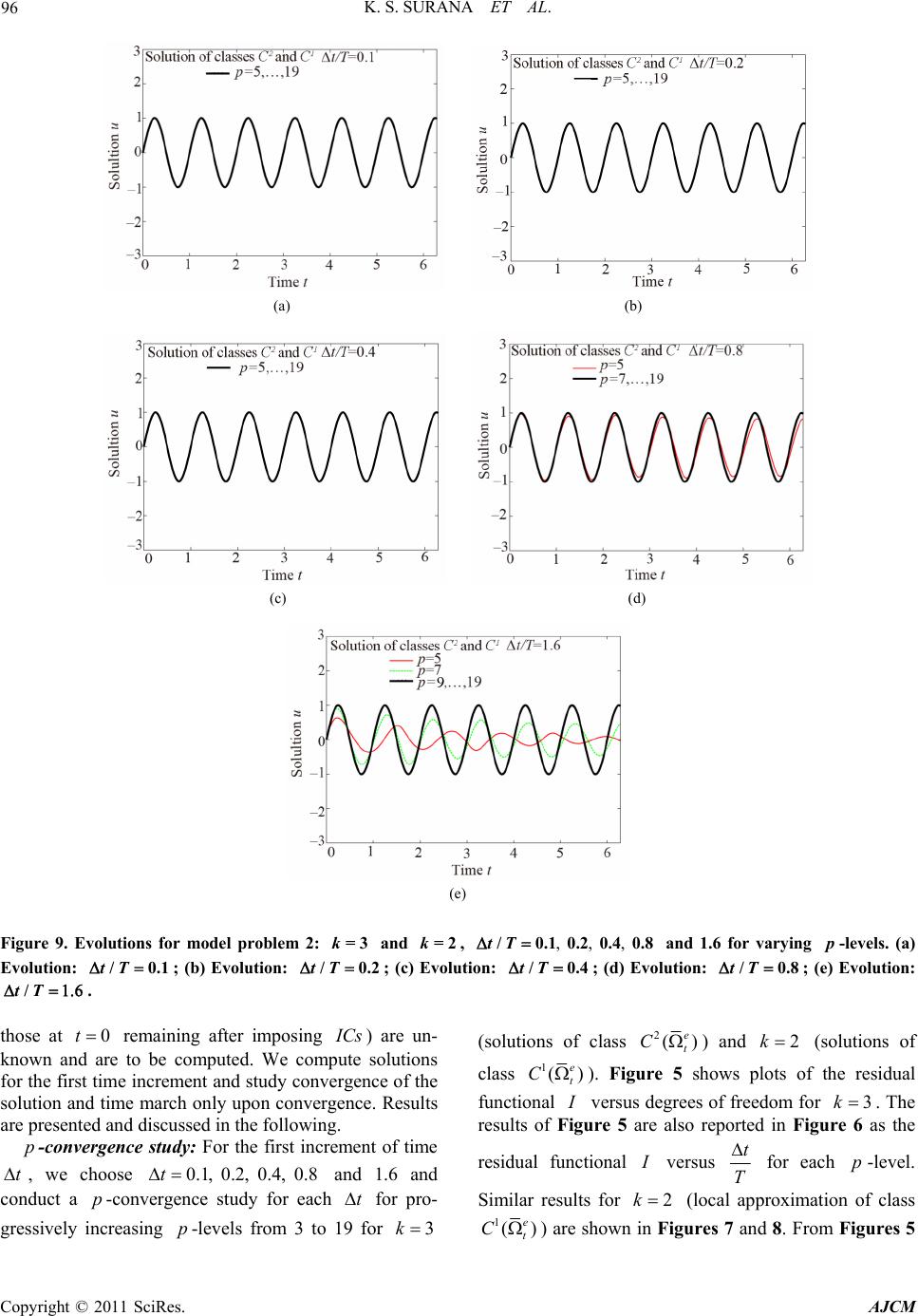 K. S. SURANA ET AL. Copyright © 2011 SciRes. AJCM 96 (a) (b) (c) (d) (e) Figure 9. Evolutions for model problem 2: =3k and =2k, , , , /0.1 0.20.40.8tT and 1.6 for varying -levels. (a) Evolution: /0.1tT; (b) Evolution: /0.2tT; (c) Evolution: /0.4tT ; (d) Evolution: /0.8tT; (e) Evolution: /tT. those at 0t remaining after imposing Cs ) are un- known and are to be computed. We compute solutions for the first time increment and study convergence of the solution and time march only upon convergence. Results are presented and discussed in the following. p-convergence study: For the first increment of time t, we choose 0.1, 0.2, 0.4, 0.8t and 1.6 and conduct a p-convergence study for each t for pro- gressively increasing p-levels from 3 to 19 for 3k (solutions of class 2() e t C ) and 2k (solutions of class 1() e t C ). Figure 5 shows plots of the residual functional versus degrees of freedom for 3k . The results of Figure 5 are also reported in Figure 6 as the residual functional versus t T for each p-level. Similar results for 2k (local approximation of class 1() e t C ) are shown in Figures 7 and 8. From Figures 5 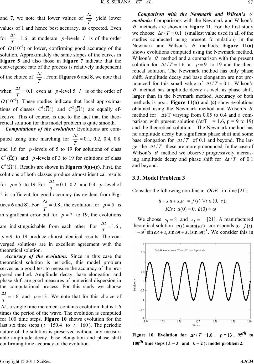 K. S. SURANA ET AL. Copyright © 2011 SciRes. AJCM 97 and 7, we note that lower values of t T yield lower values of I and hence best accuracy, as expected. Even for 1.6 t T , at moderate p-levels is of the order of O(10−6) or lower, confirming good accuracy of the solution. Approximately the same slopes of the curves in Figure 5 and also those in Figure 7 indicate that the convergence rate of the process is relatively independent of the choice of t T . From Figures 6 and 8, we note that when 0.1 t T even at p-level 5 is of the order of O(10−6). These studies indicate that local approxima- tions of classes 1() e t C and 2() e t C are equally ef- fective. This of course, is due to the fact that the theo- retical solution for this model problem is quite smooth. Computations of the evolution: Evolutions are com- puted using time marching for 0.1, 0.2, 0.4, 0.8 t T and 1.6 for p-levels of 5 to 19 for solutions of class 2() e t C and p-levels of 3 to 19 for solutions of class 1() e t C. Results are shown in Figures 9(a)-(e). First, the solutions of both classes produce almost identical results for 5p to 19. For 0.1, 0.2 t T and 0.4 p-level of 5 is sufficient for good accuracy (as evident from Fig- ures 6 and 8). For 0.8 t T , the evolution for 5p is in significant error but for 7p to 19, the evolutions are indistinguishable from each other. For 1.6 t T , 9p to 19 produce almost identical results. The con- verged solutions are in excellent agreement with the theoretical solution. Accuracy of the evolution: Since in this case the theoretical solution is periodic, this model problem serves as a good test to measure the accuracy of the pro- posed method. Amplitude decay, base elongation and phase shift are good measures of numerical dispersion in the computational process. For this study we choose 1.6 t T and 13p. We note that for this choice of t, a single time increment contains evolution that is 1.6 times the period of the wave. The evolution is computed for 100 time steps. Figure 10 shows evolution for the last six time steps (150 .4t to 160t). The periodic nature of the solution is preserved without any measur- able amplitude decay, base elongation and phase shift confirming time accuracy of the evolution. Comparison with the Newmark and Wilson’s methods: Comparisons with the Newmark and Wilson’s methods are shown in Figure 11. For the first study we choose /0.1tT (smallest value used in all of the studies conducted using present formulation) in the Newmark and Wilson’s methods. Figure 11(a) shows evolutions computed using the Newmark method, Wilson’s method and a comparison with the present solution for /1.6tT at 9p to 19 and the theo- retical solution. The Newmark method has only phase shift. Amplitude decay and base elongation are not pro- nounced for this small value of /0.1tT. Wilson’s method has amplitude decay as well as phase shift, larger than in the Newmark method. Accuracy of both methods is poor. Figure 11(b) and (c) show evolutions obtained using the Newmark method and Wilson’s method for ∆t/T varying from 0.05 to 0.4 and a com- parison with present solution (∆t/T = 1.6, p = 9 to 19) and the theoretical solution. The Newmark method has no amplitude decay but significant phase shift and some base elongation for /tT of 0.1 and beyond. The lar- ger the /tT these are more pronounced. In the case of Wilson’s method we observe progressively increas- ing amplitude decay and phase shift for /tT of 0.1 and beyond. 3.3. Model Problem 3 Consider the following non-linear ODE in time [21]: 3 12 () (0, ); : (0)0, (0) ususuftt ICs uu We choose 12s and 21s [21]. A manufactured theoretical solution ()sin( )ut t corresponds to () t 23 12 sinsin(sin )ts tst . We consider this in Figure 10. Evolution for /tT , = , 95th to 100th time steps (=3k and =2k): model problem 2. 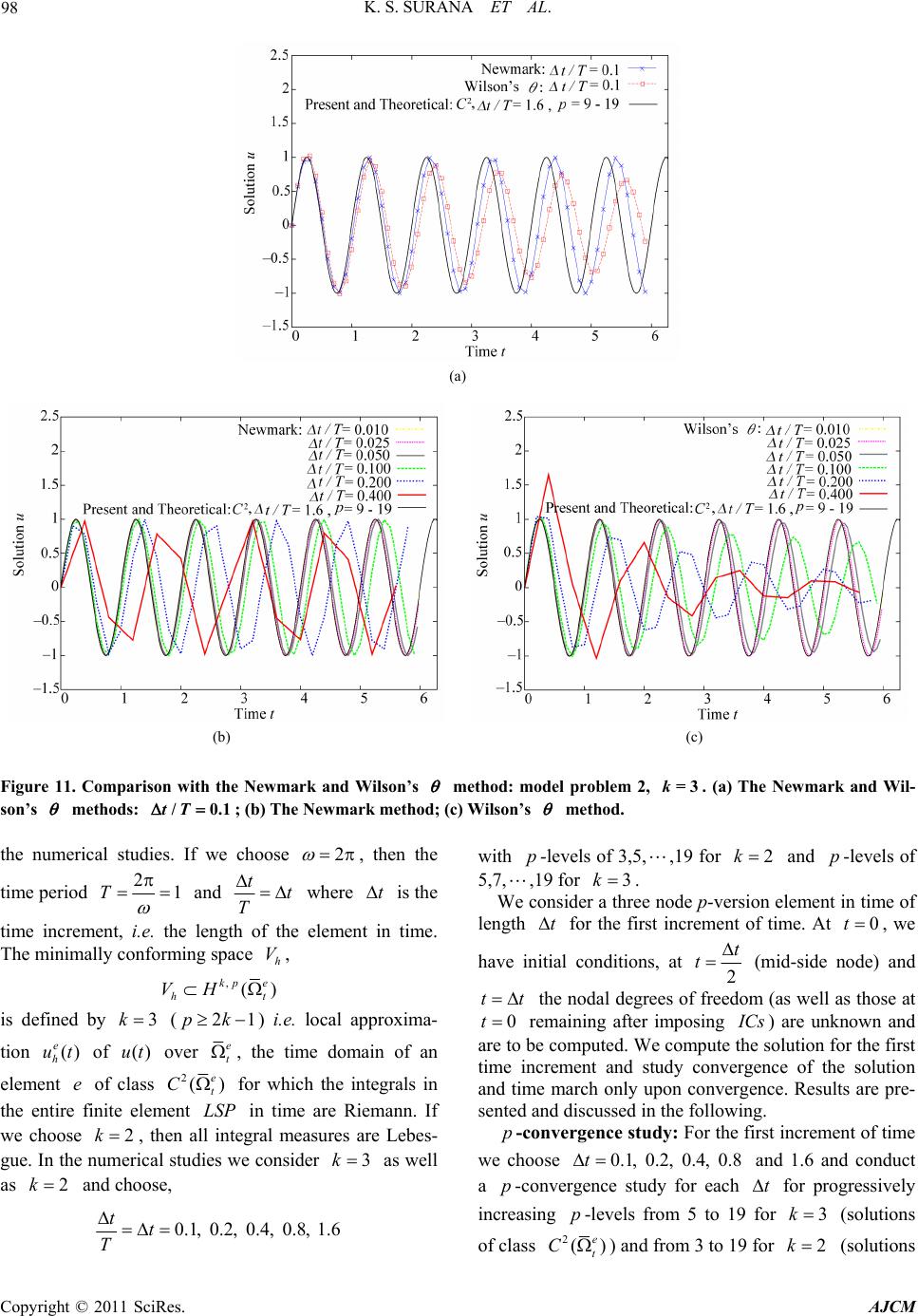 K. S. SURANA ET AL. Copyright © 2011 SciRes. AJCM 98 (a) (b) (c) Figure 11. Comparison with the Newmark and Wilson’s method: model problem 2, =3k. (a) The Newmark and Wil- son’s methods: /0.1tT; (b) The Newmark method; (c) Wilson’s method. the numerical studies. If we choose 2 , then the time period 21T and tt T where t is the time increment, i.e. the length of the element in time. The minimally conforming space h V, , () kp e ht VH is defined by 3k (21pk) i.e. local approxima- tion () e h ut of ()ut over e t , the time domain of an element e of class 2() e t C for which the integrals in the entire finite element LSP in time are Riemann. If we choose 2k, then all integral measures are Lebes- gue. In the numerical studies we consider 3k as well as 2k and choose, 0.1, 0.2, 0.4, 0.8, 1.6 tt T with p-levels of 3,5,,19 for 2k and p-levels of 5,7,,19 for 3k . We consider a three node p-version element in time of length t for the first increment of time. At 0t , we have initial conditions, at 2 t t (mid-side node) and tt the nodal degrees of freedom (as well as those at 0t remaining after imposing Cs ) are unknown and are to be computed. We compute the solution for the first time increment and study convergence of the solution and time march only upon convergence. Results are pre- sented and discussed in the following. p-convergence study: For the first increment of time we choose 0.1, 0.2, 0.4, 0.8t and 1.6 and conduct a p-convergence study for each t for progressively increasing p-levels from 5 to 19 for 3k (solutions of class 2() e t C ) and from 3 to 19 for 2k (solutions 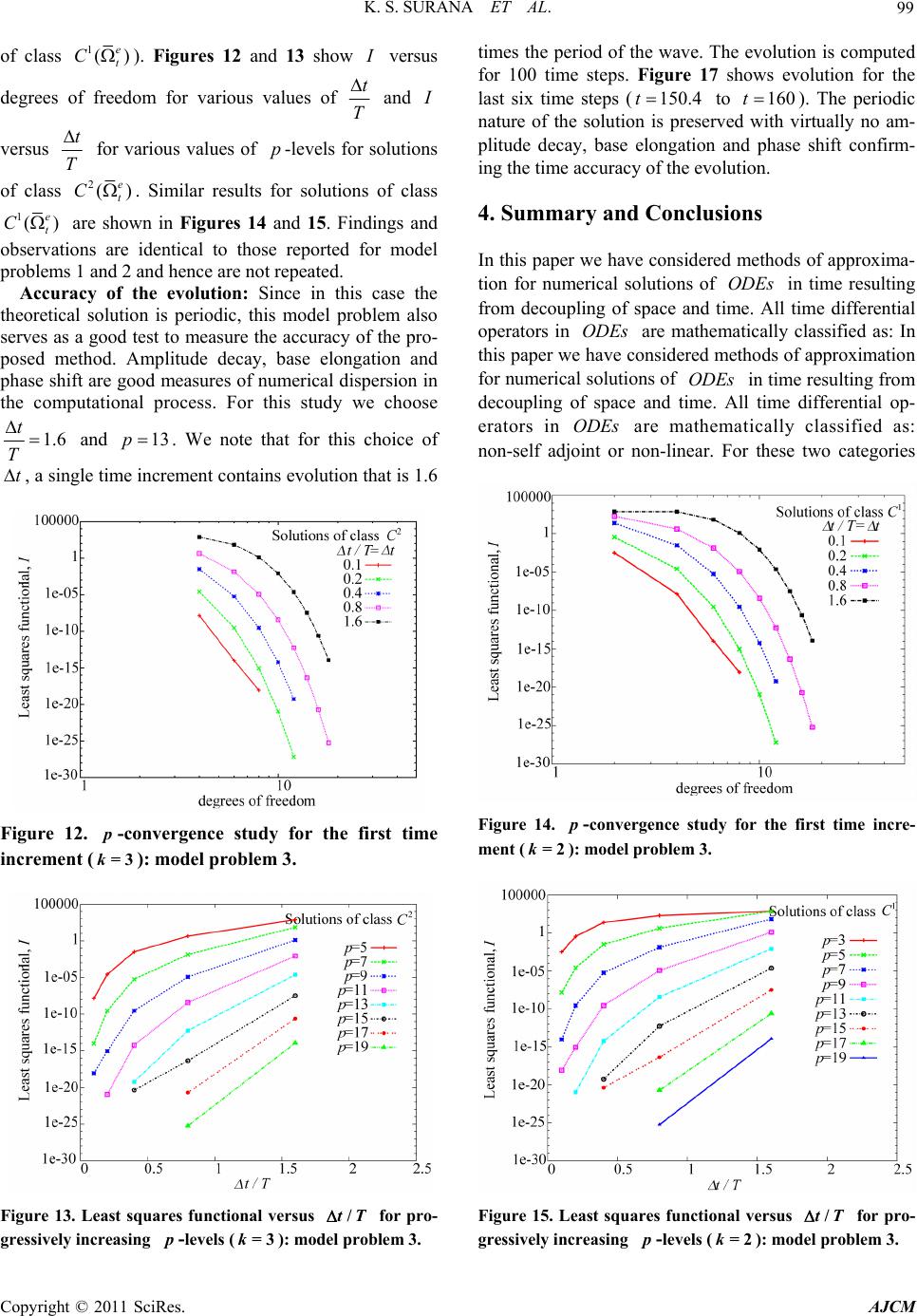 K. S. SURANA ET AL. Copyright © 2011 SciRes. AJCM 99 of class 1() e t C). Figures 12 and 13 show versus degrees of freedom for various values of t T and versus t T for various values of p-levels for solutions of class 2() e t C. Similar results for solutions of class 1() e t C are shown in Figures 14 and 15. Findings and observations are identical to those reported for model problems 1 and 2 and hence are not repeated. Accuracy of the evolution: Since in this case the theoretical solution is periodic, this model problem also serves as a good test to measure the accuracy of the pro- posed method. Amplitude decay, base elongation and phase shift are good measures of numerical dispersion in the computational process. For this study we choose 1.6 t T and 13p. We note that for this choice of t, a single time increment contains evolution that is 1.6 Figure 12. p-convergence study for the first time increment (=3k): model problem 3. Figure 13. Least squares functional versus /tT for pro- gressively increasing -levels (=3k): model problem 3. times the period of the wave. The evolution is computed for 100 time steps. Figure 17 shows evolution for the last six time steps (150 .4t to 160t). The periodic nature of the solution is preserved with virtually no am- plitude decay, base elongation and phase shift confirm- ing the time accuracy of the evolution. 4. Summary and Conclusions In this paper we have considered methods of approxima- tion for numerical solutions of ODEs in time resulting from decoupling of space and time. All time differential operators in ODEs are mathematically classified as: In this paper we have considered methods of approximation for numerical solutions of ODEs in time resulting from decoupling of space and time. All time differential op- erators in ODEs are mathematically classified as: non-self adjoint or non-linear. For these two categories Figure 14. -convergence study for the first time incre- ment (=2k): model problem 3. Figure 15. Least squares functional versus /tT for pro- gressively increasing -levels (=2k): model problem 3. 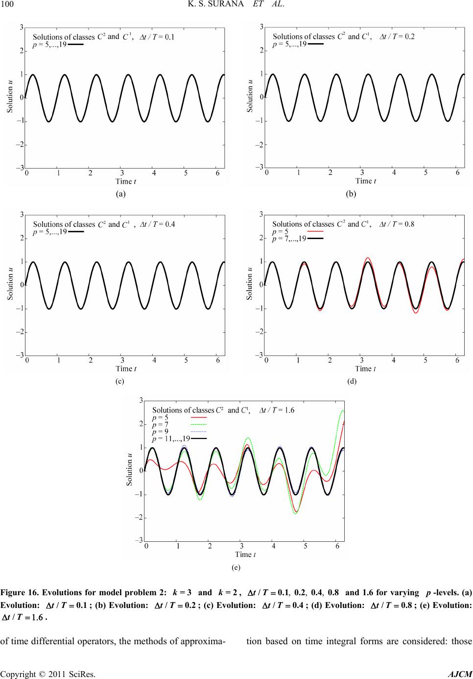 K. S. SURANA ET AL. Copyright © 2011 SciRes. AJCM 100 (a) (b) (c) (d) (e) Figure 16. Evolutions for model problem 2: =3k and = 2k, , , , /0.1 0.20.40.8tT and 1.6 for varying -levels. (a) Evolution: /0.1tT; (b) Evolution: /0.2tT; (c) Evolution: /0.4tT ; (d) Evolution: /0.8tT; (e) Evolution: /tT. of time differential operators, the methods of approxima- tion based on time integral forms are considered: those 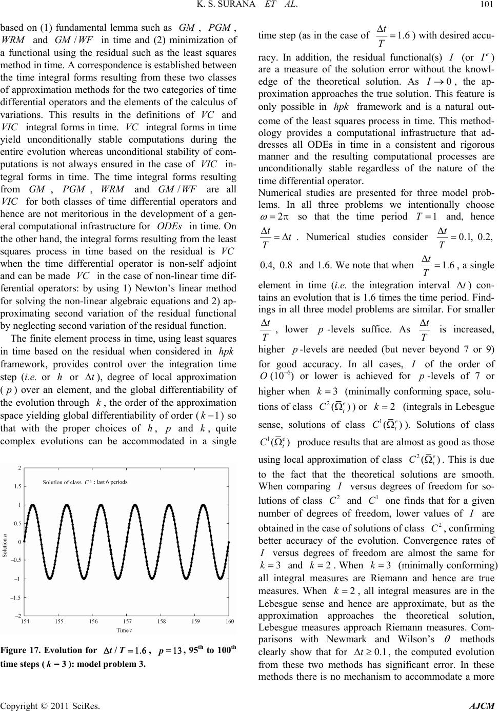 K. S. SURANA ET AL. Copyright © 2011 SciRes. AJCM 101 based on (1) fundamental lemma such as GM, PGM , WRM and /GMWF in time and (2) minimization of a functional using the residual such as the least squares method in time. A correspondence is established between the time integral forms resulting from these two classes of approximation methods for the two categories of time differential operators and the elements of the calculus of variations. This results in the definitions of VC and VIC integral forms in time. VC integral forms in time yield unconditionally stable computations during the entire evolution whereas unconditional stability of com- putations is not always ensured in the case of VIC in- tegral forms in time. The time integral forms resulting from GM , PGM , WRM and /GMWF are all VIC for both classes of time differential operators and hence are not meritorious in the development of a gen- eral computational infrastructure for ODEs in time. On the other hand, the integral forms resulting from the least squares process in time based on the residual is VC when the time differential operator is non-self adjoint and can be made VC in the case of non-linear time dif- ferential operators: by using 1) Newton’s linear method for solving the non-linear algebraic equations and 2) ap- proximating second variation of the residual functional by neglecting second variation of the residual function. The finite element process in time, using least squares in time based on the residual when considered in hpk framework, provides control over the integration time step (i.e. or h or t), degree of local approximation (p) over an element, and the global differentiability of the evolution through k, the order of the approximation space yielding global differentiability of order (1k ) so that with the proper choices of h, p and k, quite complex evolutions can be accommodated in a single Figure 17. Evolution for /tT, p=, 95th to 100th time steps (=3k): model problem 3. time step (as in the case of 1.6 t T ) with desired accu- racy. In addition, the residual functional(s) (or e ) are a measure of the solution error without the knowl- edge of the theoretical solution. As 0I, the ap- proximation approaches the true solution. This feature is only possible in hpk framework and is a natural out- come of the least squares process in time. This method- ology provides a computational infrastructure that ad- dresses all ODEs in time in a consistent and rigorous manner and the resulting computational processes are unconditionally stable regardless of the nature of the time differential operator. Numerical studies are presented for three model prob- lems. In all three problems we intentionally choose 2 so that the time period 1T and, hence tt T . Numerical studies consider 0.1, 0.2, t T 0.4, 0.8 and 1.6. We note that when 1.6 t T , a single element in time (i.e. the integration interval t ) con- tains an evolution that is 1.6 times the time period. Find- ings in all three model problems are similar. For smaller t T , lower p-levels suffice. As t T is increased, higher p-levels are needed (but never beyond 7 or 9) for good accuracy. In all cases, of the order of O(10–6) or lower is achieved for p-levels of 7 or higher when 3k (minimally conforming space, solu- tions of class 2() e t C ) or 2k (integrals in Lebesgue sense, solutions of class 1() e t C). Solutions of class 1() e t C produce results that are almost as good as those using local approximation of class 2() e t C. This is due to the fact that the theoretical solutions are smooth. When comparing versus degrees of freedom for so- lutions of class 2 C and 1 C one finds that for a given number of degrees of freedom, lower values of are obtained in the case of solutions of class 2 C, confirming better accuracy of the evolution. Convergence rates of versus degrees of freedom are almost the same for 3k and 2k . When 3k (minimally conforming) all integral measures are Riemann and hence are true measures. When 2k , all integral measures are in the Lebesgue sense and hence are approximate, but as the approximation approaches the theoretical solution, Lebesgue measures approach Riemann measures. Com- parisons with Newmark and Wilson’s methods clearly show that for 0.1t , the computed evolution from these two methods has significant error. In these methods there is no mechanism to accommodate a more  K. S. SURANA ET AL. Copyright © 2011 SciRes. AJCM 102 complex evolution in a time step than that corresponding to linear acceleration. Hence, for better accuracy there is no other alternative but to reduce the integration time step. In the present approach, the minimally conforming choice of k with progressively increasing p-levels permits accurate computation of more and more complex evolutions for a fixed increment of time. Numerical studies presented for model problems 2 and 3 for 100 time steps with 1.6 t T at 13p, confirm that the evolution remains free of amplitude decay, base elonga- tion and phase shift. Similar computations using New- mark method or Wilson’s method with reasonable accuracy (but worse than the present approach) would require 0.0 5 t T , i.e. 3200 time steps. In conclusion, the methodology presented here ad- dresses all ODEs in time in a uniform and rigorous manner without any special and application dependent adjustments, yields unconditionally stable computations during the entire evolution, has a built in mechanism of error measure without the knowledge of theoretical solu- tion, permits large time steps while maintaining desired accuracy of the evolution, and is free of amplitude decay, base elongation and phase shift for large t T (with roper choices of k and p) and, hence is highly meritorious. 5. Acknowledgements The financial support provided to the second author by Honeywell Federal Manufacturing & Technologies th- rough employment is greatly appreciated. The third au- thor (JNR) acknowledges the research was carried out while the author was supported by AFOSR Grant FA9550-09-1-0686. The support to the first (KSS) and third (JNR) authors through their endowed professor- ships is also greatly appreciated. The use of computa- tional facilities in the Computational Mechanics Labora- tory (CML) at the University of Kansas are also ac- knowledged. 6. References [1] M. Gelfand and S. V. Foming, “Calculus of Variations,” Dover, New York, 2000. [2] S. G. Mikhlin. “Variational Methods in Mathematical Physics,” Pergamon Press, New York, 1964. [3] J. N. Reddy, “Functional Analysis and Variational Meth- ods in Engineering,” McGraw-Hill, New York, 1986. [4] J. N. Reddy, “Energy Principles and Variational Methods in Applied Mechanics,” 2nd Edition, John Wiley, New York, 2002. [5] C. Johnson, “Numerical Solution of Partial Differential Equations by Finite Element Method,” Cambridge Uni- versity Press, Cambridge, 1987. [6] T. Belytschko and T. J. R. Hughes, “Computational Methods in Transient Analysis,” North-Holland, 1983. [7] T. J. R. Hughes and T. Belytschko. “A Precis of Devel- opments in Computational Methods for Transient Analy- sis,” Journal of Applied Mechanics, Vol. 50, No. 4a, 1983, 1033-1041. doi:10.1115/1.3167186 [8] Nathan M. Newmark. “A Method of Computation for Structural Dynamics,” Journal of the Engineering Me- chanics Division, Vol. 85, No. EM3, 1959, pp. 67-94. [9] K. J. Bathe and E. L. Wilson, “Numerical Methods in Finite Element Analysis,” Prentice Hall, New Jersey, 1976. [10] W. L. Wood, M. Bossak, and O. C. Zienkiewicz, “An Alpha Modification of Newmark’s Method,” Interna- tional Journal for Numerical Methods in Engineering, Vol. 15, No. 10, 1980, pp. 1562-1566. doi:10.1002/nme.1620151011 [11] M. Hans, J. Hilber, Thomas, R. Hughes and L. Robert Taylor, “Improved Numerical Dissipation for Time Inte- gration Algorithms in Structural Dynamics,” Earthquake Engineering and Structural Dynamics, Vol. 5, No. 3, 1977, 283-292. doi:10.1002/eqe.4290050306 [12] J. Chung and G. M. Hulbert, “A Time Integration Algo- rithm for Structural Dynamics with Improved Numerical Dissipation: The Generalized- Method,” Journal of Applied Mechanics, Vol. 60, No. 2, 1993, pp. 371-375. doi:10.1115/1.2900803 [13] V. A. Leontiev, “Extension of LMS Formulations for L- Stable Optimal Integration Methods with U0-V0 Over- shoot Properties in Structural Dynamics: The Level-Symmetric (LS) Integration Methods,” Interna- tional Journal for Numerical Methods in Engineering, Vol. 71, No. 13, 2007,pp. 1598-1632. doi:10.1002/nme.2008 [14] S. Erlicher, L. Bonaventura and O. S. Bursi, “The Analy- sis of the Generalized- Method for Non-Linear Dy- namic Problems,” Computational Mechanics, Vol. 28, No. 2, 2002, pp. 83-104. doi:10.1007/s00466-001-0273-z [15] D. Kuhl and M. A. Crisfield, “Energy-Conserving and Decaying Algorithms in Non-Linear Structural Dynam- ics,” International Journal for Numerical Methods in En- gineering, Vol. 45, No. 5, 1999, pp. 569-599. doi:10.1002/(SICI)1097-0207(19990620)45:5<569::AID- NME595>3.0.CO;2-A [16] K. K. Tamma, X. Zhou and D. Sha. “A Theory of De- velopment and Design of Generalized Integration Opera- tors for Computational Structural Dynamics,” Interna- tional Journal for Numerical Methods in Engineering, Vol. 50, No. 7, 2001, pp. 1619-1664. doi:10.1002/nme.89 [17] K. K. Tamma and R. R. Namburu. “Applicability and Evaluation of an Implicit Self-Starting Unconditionally Stable Methodology for the Dynamics of Structures,” Computers and Structures, Vol. 34, No. 6, 1990, pp. 835-842. doi:10.1016/0045-7949(90)90354-5 [18] X. Zhou and K. K. Tamma, “Design, Analysis, and Syn-  K. S. SURANA ET AL. Copyright © 2011 SciRes. AJCM 103 thesis of Generalized Single Step Single Solve and Opti- mal Algorithms for Structural Dynamics,” International Journal for Numerical Methods in Engineering, Vol. 59: No. 5, 2004, pp. 597-668. doi:10.1002/nme.873 [19] X. Zhou and K. K. Tamma. “Algorithms by Design With Illustrations to Solid and Structural Mechanics/Dyna- mics,” International Journal for Numerical Methods in Engineering, Vol. 66, No. 11, 2006, pp. 1738-1790. doi:10.1002/nme.1559 [20] X. Zhou and K. K. Tamma. “A New Unified Theory Un- derlying Time Dependent Linear First-Order Systems: A Prelude to Algorithms by Design,” International Journal for Numerical Methods in Engineering, Vol. 60, No. 10, 2004, pp. 1699-1740. doi:10.1002/nme.1019 [21] A. Hoitink, S. Masuri, X. Zhou and K. K. Tamma, “Al- gorithms by Design: Part I – on the Hidden Point Collo- cation within LMS Methods and Implications for Nonlin- ear Dynamics Applications,” International Journal for Computational Methods in Engineering Science and Me- chanics, Vol. 9, No. 6, 2008, pp. 383-407. doi:10.1080/15502280802365873 [22] K. K. Tamma, X. Zhou and D. Sha, “The Time Dimen- sion: A Theory Towards the Evolution, Classification, Characterization and Design of Computational Algo- rithms for Transient/Dynamic Applications,” Archives of Computational Methods in Engineering, Vol. 7, No. 2, 2000, pp. 67-290. doi:10.1007/BF02736209 [23] K. S. Surana and J. N. Reddy, “Mathematics of Computa- tions and Finite Element Method for Boundary Value Problems,” ME 861 class notes. University of Kansas, Department of Mechanical Engineering, Manuscript of textbook in preparation, 2010. [24] K. S. Surana, “Mathematics of Computations and Finite Element Method for Initial Value Problems,” ME 862 class notes, University of Kansas, Department of Me- chanical Engineering, Manuscript of textbook in prepara- tion, 2010. [25] K. S. Surana, A. Ahmadi and J. N. Reddy, “k-Version of Finite Element Method for Non-Linear Differential Op- erators in BVP,” International Journal of Computational Engineering Science, Vol. 5, No. 1, 2004, pp. 133-207. doi:10.1142/S1465876304002307 [26] K.S. Surana, J. N. Reddy and S. Allu, “The k-Version of Finite Element Method for Initial Value Problems: Mathematical and Computational Framework,” Interna- tional Journal of Computational Methods in Engineering Science and Mechanics, Vol. 8, No. 3, 2007, pp. 123-136. doi:10.1080/15502280701252321 [27] K. S. Surana, S. Allu, J. N. Reddy and P. W. Tenpas, “Least Squares Finite Element Processes In Hpk Mathe- matical Framework for Non-Linear Conservation Law,” International Journal of Numerical Methods in Fluids, Vol. 57, No. 10, 2008, pp. 1545-1568. doi:10.1002/fld.1695 [28] B. C. Bell and K. S. Surana, “p-Version Least Squares Finite Element Formulation of Two Dimensional Incom- pressible Non-Newtonian Isothermal and Non-Isothermal Fluid Flow,” International Journal of Numerical Methods in Fluids, Vol. 18, No. 2, 1994, pp. 127-167. doi:10.1002/fld.1650180202 [29] B. C. Bell and K. S. Surana. A Space-Time Coupled P-Version LSFEF for Unsteady Fluid Dynamics, Interna- tional Journal for Numerical Methods in Engineering, Vol. 37, No. 20, 1994, pp. 3545-3569. doi:10.1002/nme.1620372008 [30] D. L. Winterscheidt and K. S. Surana, “p-Version Least Squares Finite Element Formulation for Two Dimen- sional Incompressible Fluid Flow,” International Journal of Numerical Methods in Fluids, Vol. 18, No. 1, 1994, pp. 43-69. doi:10.1002/fld.1650180104 [31] D. L. Winterscheidt and K. S. Surana, “p-Version Least Squares Finite Element Formulation for Burgers Equa- tion,” International Journal for Numerical Methods in Engineering, Vol. 36, No. 21, 1993, pp. 3629-3646. doi:10.1002/nme.1620362105 [32] K. S. Surana, A. Ahmadi and J. N. Reddy, “k-Version of Finite Element Method for Self-Adjoint Operators in BVP,” International Journal of Computational Engi- neering Science, Vol. 3, No. 2, 2002, pp. 155-218. doi:10.1142/S1465876302000605 [33] K. S. Surana, A. Ahmadi, and J. N. Reddy, “k-Version Of Finite Element Method for Non-self-adjoint Operators in BVP,” International Journal of Computational Engi- neering Science, Vol. 4, No. 4, 2003, pp. 737-812. doi:10.1142/S1465876303002179
|