 Journal of Power and Energy Engineering, 2015, 3, 97-105 Published Online April 2015 in SciRes. http://www.scirp.org/journal/jpee http://dx.doi.org/10.4236/jpee.2015.34015 How to cite this paper: Cheung, K.W. and Wu, J. (2015) Towards Optimal Transmission Switching in Day-Ahead Unit Com- mitment. Journal of Power and Energy Engineering, 3, 97-105. http://dx.doi.org/10.4236/jpee.2015.34015 Towards Optimal Transmission Switching in Day-Ahead Unit Commitment Kwok W. Cheung, Jun Wu Alstom Grid, Inc., Redmond, Washington, USA Email: kwok.cheung@alstom.com, jun.x.wu @alstom.com Received Dec emb er 2014 Abstract Co-optimizing transmission topology with generation dispatch, and leveraging grid controllability could be a viable way to improve economic efficiency of system operations in control centers. In particular, day-ahead unit commitment is a typical business process that electric utilities deploy to ensure enough generation capacity is committed day-ahead to meet the load for the next day. In a market environment, day-ahead reliability unit commitment (DA-RUC) performs a simultaneous solution of minimizing the cost of commitment for resources to meet forecasted load, net sche- duled interchange and operating reserve requirements using security constrained unit commit- ment (SCUC). The commitment may then be further checked by running security constrained eco- nomic dispatch (SCED) to verify that the commitment solution can be feasibly dispatched subject to system constraints and activated transmission constraints for each hour identified in the study period. This paper applies Optimal Transmission Switching (OTS) in DA-RUC using some heuristic pre-screening techniques to reduce the dimension of the OTS problem. Various pre-screening method s of candidate transmission lines for switching are proposed and compared. Simulation results will be presented to demonstrate generation dispatch combined with OTS in each hour could reduce congestion cost and significantly lower generation cost. Keywords Transmission Switching, Market Efficiency, System Operation, Economic Dispatch 1. Introduction The restructured electric power industry has brought new challenges for the secured and efficient operation of stressed power systems. In North America, almost all Regional Transmission Organizations (RTO) such as PJM, Midcontinent ISO or ISO New England, are fundamentally reliant on wholesale market mechanism to optimally dispatch energy and ancillary services of generation resources reliably over large geographical regions [1] [4]. A typical market system in North America supports a series of business functions for market and system opera- tions. Depending on operational needs, the system can be configured to include one or more of the following business processes (Figure 1). Reliability Unit Commitment (RUC) process provides system operators a set of tools to revise the day-ahead unit commitment schedule as necessary in order to ensure that the forecasted load and operating reserve 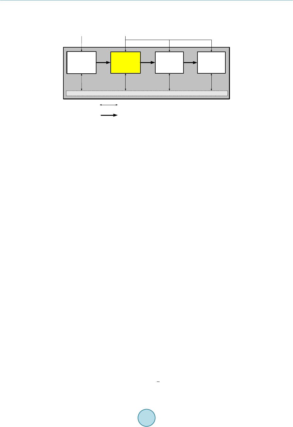 K. W. Cheung, J. Wu Reliability Unit Commitment Real-Time M ar ket Look-Ahead Commitment and Dispatch Day-Ahead M ar ket DAM Offers, Bid and Operating Reserve Requirem ents RTM Offers/ cost curves, Load Forecast and Operating Reserve Requirem ents Comprehensive Operating Plan Data flow Business process flow Figure 1. Business processes of a market system. requirements will be met and the transmission system is reliable and secured. The RUC performs a co-optimized simultaneous solution to minimize the cost of commitment for resources to meet forecasted load, net scheduled interchange and operating reserve requirements using SCUC. The commitment may then be further confirmed by running SCED to verify that the commitment solution can be feasibly dispatched subject to system con- straints and activated transmission constraints for each hour in the study period. In recent years, energy systems whether in developed or emerging economies are undergoing changes due to the challenges imposed by smart grid. Optimal transmission switching [2] [3] seems to be a viable way to leve- rage grid controllability for enhancing system performance. Transmission control has been identified as a valua- ble mechanism for a variety of benefits, from improving the system reliability, stability to improving the market surplus and efficiency of the grid. It is obvious that transmission systems could become smarter and more efficient when the control of network topology can be factored into the overall dispatch process of generation and transmission resources taking both system reliability and economics into consideration in a systematic fashion. The problem of OTS can be formu- lated as a mixed-integer programming problem. However, it requires the introduction of a significant number of integer variables for transmission line in/out statuses which becomes a key impediment of applying a full OTS scheme in any large power network. Fortunately, a practical solution to improve operational efficiency could be achieved by limiting the set of transmission line candidates for OTS. The rest of the paper will be presented as follows. Section 3 addresses the basic model of OTS. Section 4 proposes selection methods of candidate transmission lines for a study of OTS in DA-RUC. Section 5 presents numerical results for the DA-RUC/SCED using OTS for a large-scale power system with more than 37,000 buses. Conclusions are in Section 6. 2. OTS Modeling The core application of the market system is basically a centralized market clearing engine solving a unit com- mitment, scheduling and dispatch problem. The problem itself is typically formulated as a Mixed Integer Pro- gramming (MIP) problem [5]. A compact of form of such problem can be described as follows: ( ) ( ) ( ) ( ) 1 , min , gt gtgtgtgt gt gt u puu χς − + ∑ (1) Subject to (2) (3)  K. W. Cheung, J. Wu , , gt gtgtgt gt up pupgt ≤≤ ∀ (4) (5) (6) , , kt ktktkt kt fz ffzkt≤≤ ∀ (7) ()( ) , 10 , mn mtntktktk Bfz Mkt θθ −− +−≥∀ (8) ()() , 10 , mn mtntktktk Bfz Mkt θθ −− −−≤∀ (9) ( ) 1 _Open, , kt k z jkt−≤ ∀ ∑ (10 ) (11 ) to loss line line ,, fr mm gmt mtmtktkt kk plpffmt ∈∈ −− =−∀ ∑∑ (12) ( ) 1, , gtgt gt gt ppu Rgt − −≤ ∀ ( 13) (14) where m and n are “from” and “to” bus of transmission line k, respectively, and listed in (7)-(10) is the bi- nary variable representing the state of the transmission element; a value of 1 reflects a closed status and a value of 0 reflects an open status. listed in (8) and (9) is an arbitrarily large number. When the binary variable is 1, the value of is irrelevant. When the binary variable is 0, the value of should be big enough to ensure that (8) and (9) are satisfied regardless of the difference in the bus angles. For all practical purposes can be set to . j_Ope n listed in (10) denotes the maximum number of open lines. The objective (1) is to minimize the production plus start-up costs. The minimization is subject to many con- straints including supply and demand constraints (2), capacity constraints (4), (5), (6), ramp constraints (13), transmission constraints with transmission line switching (7), (8), (9), (10), (11), bus node power balance (12) and reserve requirements (3). It is important to note that the transmission flow can also be expressed as a linear function of bus net injections in the pre-contingent state. (15) Most RTO’s real-time operation requires the n-1 security. Hence, the transmission flow presented here can either be pre-contingent or post-contingent line or interface flow. Other constraints, such as minimum up and down times constraints, ramp constraints, and operating and regulating etc. reserve requirements are considered as a part of (14). After the unit commitment problem is solved, the integer variables will be frozen, the optimal solution for the scheduling and dispatch problem will be reduced to a Linear Programming (LP) problem in which mar- ket clearing quantities and market clearing prices by location can be determined. The market clearing prices by location, called locational marginal prices are by-products of the optimization solution. Locational marginal prices for energy can be written as: loss LMP t gtttkgt kt k gt pa p λλ µ ∂ =−− ∂ ∑ (16) The three terms in the above LMP equation could be interpreted as the three components of LMP namely ener gy, loss and congestion, respectively. These locational price results give precise representation of the cause-effect relationship that is consistent with grid reliability management. 3. Transmission Line Switching Selection With the introduction of in the OTS model, transmission switching adds substantial computational com-  K. W. Cheung, J. Wu plexity to the market clearing engine. To be able to solve the MIP model for large scale systems, transmission lines are divided into two sets. One is a set of switchable transmission lines which are associated with decision integer variables as in (7)-(10). The other is a set of transmission lines which status (on/off) is predetermined before running optimization of market clearing. The proper size of switchable transmission lines and the value of j_Open in (10) are critical parameters that affect solution time. These parameters might vary from networks to networks and cases by cases. [6] has shown that solving OTS could be done within the required time in large electricity market systems by selecting a proper size of candidate transmission lines. However, it remains as a challenge on how to select a proper set of candi- date transmission lines to get better objective savings among thousands of transmission lines for a given large- scale power system. With a given limit of switchable transmission lines, the following criteria are proposed to be used for the selection of switchable transmission lines. 3.1. Selection Criteria 3.1.1. Limit Violations of Transmission Lines For a given base case, if transmission lines violated their limits, the violation penalties will appear in the cost of the objective function. Switching off the violated transmission lines that does not cause any new violations will eliminate the high penalty costs introduced by those violated transmission lines. Hence, the violated transmis- sion lines could be good candidates of switchable transmission lines. 3.1.2. Binding Transmission Lines For a given base case, binding transmission lines are the resources to cause congestion and lead to dispatching more expensive generation. Switching off binding transmission lines that does not cause other lines to be con- gested could reduce congestion cost. Hence, binding transmission lines could also be good candidates of switch- able transmission lines. 3.1.3. Congestion Rents of Transmission Lines Congestion rent (CR) [7] [9], which is defined as the difference in shadow prices between “from” and “to” side bus of a transmission line k, multiplied by the flow on the line. (17) By introducing a fictitious variable of “fraction of line out of service” [8] suggested to use (17) to rank trans- mission lines for switching. Due to complementary slackness, the shadow price of a transmission line is zero if there are no transmission constraints binding; negative if there are transmission constraints binding at upper lim- its; positive if there are transmission constraints binding at lower limits. The lines are congested when there are shadow price differences between “from” and “to” side of the line of interest. Switching off these transmission lines would possibly reduce the congestion costs. 3.1.4. Production Costs Associated with Transmission Lines The production cost (PC) could be increased due to transmission congestion. In those cases, some higher-cost generation is dispatched in favor of lower-cost generation that would otherwise be used in the absence of trans- mission constraints. In our previous research work [10], a formulation of the sensitivities of bus angle with respect to the flow of transmission line is developed: ( ) 11 it ikmn mini kt B f θβ −− ∂==Π −Π ∂ (18) where elements of matrix : 22 , iiijij ij ji BB ≠ Π= Π=− ∑ (19) The production cost associated with the transmission line k is PCkgthh hkhi ikk g ih cBB f ββ ≠ = − ∑∑ (20)  K. W. Cheung, J. Wu whe r e denotes the energy offer price of generator g at time t and h denotes the bus to which generation g is connected. Intuitively, if the transmission line k is congested, switching it off will cause to go to 0. If switching off line k does not cause more congestion on other lines, it will reduce the overall congestion cost. Thus PC asso- ciated with transmission line can be used as another selection criterion for transmission switching candidates. 3.2. Selection Methods of Switchable Lines The purpose of selecting candidate transmission lines for switching is to identify those transmission lines which could eliminate or reduce congestion cost for a given power network. For all practical purposes, the OTS prob- lem could be solved by selecting one candidate line at a time or limiting the maximum number of open lines. In either case, a proper size of candidate set of transmission lines [6] is crucial to make the problem tractable. Table 1 illustrates OTS solver solution time for different size of candidate transmission lines (OTSbr) and different maximum number of open lines j_Open. From Table 1, a practical number of switchable transmission lines are probably less than 20 and the maximum number of open lines j_Open is about 10. Tractable values of OTSbr and j_Open could vary with the size of power network. However, these parameters usually do not vary much for a given power network and can be determined via offline studies. The violated transmission lines, if any, will first be selected as switching candidates since they usually cause large penalty costs in the objective function. However, this criterion is usually not satisfied under normal system conditions. Instead, binding transmission constraints are more likely to be observed. Both CR and PC can be used as ranking measures for effective transmission switching candidates. However, combining PC and CR (PCCR) [10] could more effectively reduce overall objective cost. It is important to note that neither CR, PCCR, nor binding transmission lines by itself is a perfect measure since they are all topology-dependent. In other words, there is no guarantee that new congestion will not occur when topology changes. Therefore, in the RUC/SCED OTS study, we propose to use the following methods to select candidate transmission lines: 1) OTS_CR—Rank transmission lines by congestion rent (CR), and select the higher ranking transmission lines as candidate transmission lines. 2) OTS _P CCR—Filter out transmission lines with non-positive , rank filtered transmission lines by CR, and select the higher ranking transmission lines as candidate transmission lines. 3) OTS_binding_CR—Rank binding transmission lines by CR and select the higher ranking transmission lines that are binding as candidate transmission lines before selecting the non-binding ones. 4) OTS _bind ing_ P C CR—Rank binding transmission lines by PCCR and select the higher ranking transmis- sion lines that are binding as candidate transmission lines before selecting the non-binding ones. 4. OTS Simulation Results We applied OTS to the DA-RUC process for one of the largest market systems in North America with more than 37,000 buses and 48,000 transmission lines. • DA-RUC Case and SCED Objective Cost w/o OTS The hourly load forecast, the number of binding transmission constraints and the objective costs of a 24 hr DA-RUC case as a baseline solution (without OTS) are shown in Table 2. Hour 4 has the lowest load, hours 12 to 21 are the high load period. Hour 4 has the least number of binding transmission constraints equal to 16 and Table 1. Solution time varies with OTSbr and j_Open. OTSbr j_Open Open Lines Solution Time (sec) 14 10 1 351 18 8 4 378 18 18 4 378 27 5 4 516 74 5 5 920 340 5 1 2444  K. W. Cheung, J. Wu Table 2. Hourly load forecast, number of binding constraints & objective cost for a DA RUC study case. Hour (h) Load (Mw) Number of Binding Constraints Objective ($/h) 1 48,640 20 847453.2 2 46,577 20 810258.7 3 45358.3 18 784169.9 4 44837.9 16 776758.6 5 45217.2 18 786803.7 6 46350.2 17 808562.2 7 47854.9 20 843179.1 8 50048.8 24 907384.6 9 53053.4 24 1009595 .5 10 55290.6 22 1200858.8 11 56437.1 24 1213839.6 12 56955.7 23 1292906.6 13 57224.9 22 1262689.1 14 57283.8 24 1190398.7 15 57,213 24 1198609.9 16 57356.2 28 1205419.0 17 57477.8 26 1222535.2 18 57268.2 27 1213888.9 19 56610.3 26 1192487.8 20 57332.1 29 1260312.3 21 57213.5 28 1286752.8 22 54646.3 25 1178705.5 23 51117.7 21 1080567.1 24 47,814 21 994112.2 hour 20 has the highest number of binding transmission constraints equal to 29. The total objective cost for the whole day is $25,568,249. • DA RUC SCED OTS Results and Analysis A group candidate transmission lines with a limit of 10 switchable candidate transmission lines is selected for each proposed method. Their simulation results of OTS are presented in Table 3. Figure 2 depicts hourly objective costs for the proposed methods. In general, the objective savings during the peak hours starting from hour 9 are more than that in the valley hours between hours 1 to 8. Comparing to the baseline solution (w/o OTS), it is interesting to note that OTS objective costs are reduced for all hours except for hour 12 of OTS_binding_CR. Table 4 illustrates the total 24 hour objective cost for each method. OTS_PCCR achieves on average more objective savings in most hours compared to the rest of the other methods. 5. Conclusions Optimal transmission switching can leverage grid controllability for enhancing system performance. Due to the scale of the problem, a limited set of transmission switching candidates are pre-selected for switching by an co-optimization algorithm of energy and network topology for all practical purposes. First, simulation results from a large network in the DA- RUC demonstrate that OTS provides more savings during the peak hours of a  K. W. Cheung, J. Wu Table 3 . Comparison of objective costs. Hr Objecti ve ($/h) w/o OTS OTS-CR OTS-PCCR OTS_binding PCCR OTS_binding CR 1 847,453 845,754 844,072 844,913 845,297 2 810,259 806,667 805,545 806,869 809,141 3 784,170 780,201 779,196 780,862 783,403 4 776,759 772,239 771,687 772,567 776,207 5 786,804 781,886 781,215 782,799 786,222 6 808,562 803,937 803,922 804,449 807,356 7 843,179 838,381 838,658 837,788 842,179 8 907,385 889,834 890,768 904,569 906,945 9 1,009,596 991,478 991,434 971,654 1,004,996 10 1,200,859 1,093,192 1,096,146 1,113,900 1,192,598 11 1,213,840 1,115,292 1,098,780 1,205,136 1,210,633 12 1,292,907 1,240,486 1,143,344 1,262,159 1,292,906 13 1,262,689 1,230,259 1,138,566 1,232,974 1,250,874 14 1,190,399 1,109,584 1,112,472 1,166,548 1,181,088 15 1,198,610 1,141,618 1,121,518 1,170,307 1,192,757 16 1,205,419 1,164,641 1,141,122 1,174,303 1,189,568 17 1,222,535 1,128,318 1,160,128 1,196,153 1,202,415 18 1,213,889 1,205,853 1,205,983 1,098,233 1,210,899 19 1,192,488 1,136,221 1,138,401 1,176,815 1,189,683 20 1,260,312 1,175,088 1,173,320 1,235,244 1,252,684 21 1,286,753 1,151,641 1,142,653 1,282,454 1,284,152 22 1,178,705 1,093,961 1,092,866 1,170,503 1,172,846 23 1,080,567 923,572 1,003,549 1,052,823 1,076,384 24 994,112 841,332 852,076 960,907 989,619 Table 4. Total 24-hour objective cost comparison. w/o OTS OTS-CR OTS-PCCR OTS_binding PCCR OTS_binding CR 25,568,249 24,261,435 24,127,421 25, 004,929 25,450,852 Figure 2. Hourly objective cost comparison.  K. W. Cheung, J. Wu reasonably stressed system. Secondly, a smaller size of candidate transmission line requires less computation time but can still provide considerable objective savings. PC CR is likely a better selection criterion that of CR in terms of objective savings. In some cases, applying PCCR to only the binding transmission lines could be a rea- sonable compromise if computation time is a concern. References [1] Cheung, K.W. (2008) Ancillary Service Market Design and Implementation in North America: From Theory to Prac- tice. Panel Paper, Proceedings of the 3rd International Conference on Electric Utility Deregulation, Restructuring and Power Technologies (DRPT), Nanjuing, 6-9 April 2008, 66-73. http://dx.doi.org/10.1109/DRPT.2008.4523381 [2] Wood, A. J. and Wollenberg, B.F. (1996) Power Generation, Operation, and Control. 2nd Edi t io n , John Wiley & Sons, New York. [3] Fisher, E.B., O’Neill, R.P. and Ferris, M.C. (2008) Optimal Transmission Switching. IEEE Transactions on Power Systems, 23, 1343-13 55. http://dx.doi.org/10.1109/TPWRS.2008.922256 [4] Chow, J.H., deMello, R. and Cheung, K.W. (2005) Electricity Market Design: An Integrated Approach to Reliability Assuran ce. Invited P ape r , IEEE Proceeding (Special Issue on Power Technology & Policy: Forty Years after the 1965 Blackout), 93 , 1956-1969. [5] Cheung, K. W. (2011) Economic Evaluation of Transmission Outages and Switching for Market and System Opera- tions. Panel Paper, Proceedings of 2011 IEEE PES General Meeting. [6] Cheung, K.W., Wu, J. and Rios-Zalapa, R. (2010) A Practical Implementation of Optimal Transmission Switching. Proceedings of the 4th International Conference on Electric Utility Deregulation, Restructuring and Power Technolo- gies (DRPT 2010). [7] Hedman , K.W., O’Neill, R .P ., Fis h er , E.B. and Oren, S.S. (2008) Optimal Transmission Switching—Sensitivity Anal- ysis and Extensions. IEEE Transactions on Power Systems, 23, 1469-14 79 . http://dx.doi.org/10.1109/TPWRS.2008.926411 [8] Fuller, J.D., Ramasra, R. and Cha, A. (2012) Fast Heuristics for Transmission Line Switching. IEEE Transactions on Power Systems, 27, 1377-13 86. http://dx.doi.org/10.1109/TPWRS.2012.2186155 [9] Ruiz, P. A. , Foster, J.M . , Rudkevi ch , A. and Caramanis, M.C. (20 11) On Fast Transmission Topology Control Heuris- tics. Proceedings of 2011 IEEE PES General Meeting. [10] Wu, J. and Cheung, K. W. (2013 ) On Selection of Transmission Line Candidates for Optimal Transmission Switching in Large Power Networks. Proceedings of IEEE PES General Meeting, 21-25 July 2013, Vancouver, BC.  K. W. Cheung, J. Wu Nomenclature : Index for generator, : Index for study period, : Index for transmission line, : Index for “from”, “to” bus of transmission line k, , : Set of transmission lines whose “from”, “to” sides are connected to bus m, : Load forecast for system and bus m for study period t, : Capacity limits of generator g for study period t, : Reserve requirement for study period t, : Reserve limit of generator for study period t, : Ramp limit of generator for study period t, : Susceptance of transmission line, : Limit of transmission line k for study period t, : Sensitivity of transmission line k with respect to generator g for study period t, : bus angle of bus m for study period t, , : High and low limits of bus angle for study period t, : Commitment status for generator g for study period t; gt : Power output of generator g for study period t, : Reserve contribution of generator g for study period t, : Transmission line flow for study period t, : vector of all , : vector of all gt , : vector of all , : set of feasible solutions, : Production and no-load costs for generator g for study period t, : Start-up costs for generator g for study period t, : Loss for system and bus m for study period t.
|