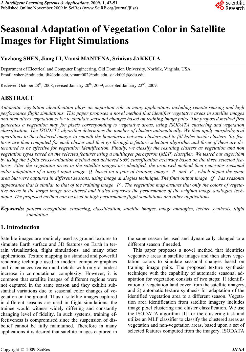J. Intelligent Learning Systems & Applications, 2009, 1, 42-51
Published Online November 2009 in SciRes (www.SciRP.org/journal/jilsa)
Seasonal Adaptation of Vegetation Color in Satellite
Images for Flight Simulations
Yuzhong SHEN, Jiang LI, Vamsi MANTENA, Srinivas JAKKULA
Department of Electrical and Computer Engineering, Old Dominion University, Norfolk, Virginia, USA.
Received October 28th, 2008; revised January 20th, 2009; accepted January 22nd, 2009.
ABSTRACT
Automatic vegetation identification plays an important role in many applications including remote sensing and high
performance flight simulations. This paper proposes a novel method that identifies vegetative areas in satellite images
and then alters vegeta tion color to simulate sea sonal chang es ba sed on tra ining imag e pairs. Th e propo sed m ethod first
generates a vegetation map for pixels corresponding to vegetative areas, using ISODATA clustering and vegetation
classification. The ISODATA algorithm determines the number of clusters automatica lly. We then apply morphologica l
operations to the clustered images to smooth the boundaries between clusters and to fill holes inside clusters. Six fea-
tures are then computed for each cluster and then go through a feature selection algorithm and three of them are de-
termined to be effective for vegetation identification. Finally, we classify the resulting clusters as vegetation and non
vegetation types based on the selected features using a multila yer perceptro n (MLP) classifier. We tested our algorithm
by using the 5-fold cross-validation method and achieved 96% classification accuracy based on the three selected fea-
tures. After the vegetation areas in the satellite images are identified, the proposed method then generates seasonal
color adaptation of a target input image based on a pair of training images and , which depict the same
area but were captured in differen t season s, using image ana logies techniqu e. The final output imag e has seasonal
appearance that is similar to that of the training image
QP P
Q
P. The vegetation map ensures that only the colors of vegeta-
tive areas in the target image are altered and it also improves the performance of the original image analogies tech-
nique. The proposed method can be used in high performance flight simulations and other applications.
Keywords: pattern recognition, clustering, classification, satellite images, image analogies, texture synthesis, flight
simulation
1. Introduction
Satellite images are routinely used as ground textures to
simulate Earth surface and 3D features on Earth in ter-
rain visualization, flight simulations, and many other
applications. Texture mapping is a standard and powerful
rendering technique used in modern computer graphics
and it enhances realism and details with only a modest
increase in computational complexity. However, it is
common that satellite images of different regions were
not captured in the same season and they exhibit sub-
stantial variations due to seasonal color changes of ve-
getation on the ground. Thus if satellite images captured
in different seasons are used in flight simulations, the
trainee would witness widely differing and constantly
changing level of fidelity. In such systems, training ef-
fectiveness is compromised since the suspension of dis-
belief cannot be fully maintained. Therefore in many
applications it is desired that satellite images captured in
the same season be used and dynamically changed to a
different season if needed.
This paper proposes a novel method that identifies
vegetative areas in satellite images and then alters vege-
tation colors to simulate seasonal changes based on
training image pairs. The proposed texture synthesis
technique with the capability of automatic seasonal ad-
aptation for vegetation consists of two steps: 1) identifi-
cation of vegetation land cover from the satellite imagery;
and 2) automatic texture synthesis for adaptation of the
identified vegetation area to a different season. Vegeta-
tion area identification from satellite imagery includes
image pixel clustering and cluster classification. We use
the ISODATA algorithm [1] for the clustering task and
utilize an MLP classifier to classify the clustered areas as
vegetation and non-vegetation areas, based upon a set of
selected features computed from the imagery. ISODATA

43 YUZHONG SHEN, JIANG LI, VAMSI MANTENA, SRINIVAS JAKKULA
is a divisive process which divides data into homogene-
ous clusters. There are two data passes in each iteration
of the ISODATA algorithm. The first pass finds the
means for each of the predefined number of clusters. The
clusters are then split and merged in the second pass,
depending upon their standard deviations, distance be-
tween means, cluster size and total number of clusters.
Once the terminating criterion has been met, each data
point is clustered into one of the predetermined clusters
in terms of their distances to the cluster means. Usually,
a post-processing step for smoothing cluster boundaries
is needed due to noise in the image [2]. We apply mor-
phological operations on the clustered images to smooth
the boundaries between clusters and to fill holes inside
clusters.
However, the ISODATA algorithm is an unsupervised
learning process and land cover types of the resulting
clusters are unknown. Therefore, the classification step is
necessary. The next step is to identify the land cov er typ e
for each of the clusters. We compute a set of statistics for
each of the clusters and train a classifier to classify the
clusters into one of the land cover types. The statistics
include mean and standard deviation of each spectral
channel of the image. Note that not all the statistics are
useful for the classification, we thus utilized a feature
selection algorithm to identify th e most effective features
for the classification.
Training unnecessarily large classifiers can have side
effects including the curse of dimensionality, conver-
gence difficulties and large validation errors. In order to
avoid these problems, feature selection is usually applied
to generate a compact subset of features that leads to an
accurate model for the given data. In feature selection,
the algorithm often evaluates the fitness of candidate
features first, it then searches for feature combinations
with the goal of maximizing the fitness value. There are
three popular different kinds of feature selection algo-
rithms: filter, wrapper and embedded. A filter approach
performs the fitness evaluation as a preprocessing step
with no classifier involved such as FOCUS [3], Fisher
criterion [4], weight-based [5] and RELIEF [6] algo-
rithms. Filter approaches are usually very efficient but
the selected feature subset may not perform well. A
wrapper approach determines the fitness of a feature
subset by actually training a classifier [7]. They usually
have better performances at the cost of higher computa-
tional complexities. In the embedded approach, feature
selection is done inside the algorithm itself. Examples
include C4.5 [8] and CART [9]. In our previous work,
we developed an efficient wrapper feature selection al-
gorithm but it is as efficient as a filter algorithm [10]. We
apply the feature selection algorithm to the six derived
features and use a classification algorithm, also devel-
oped by the authors, to automatically identify lan d cover
type of the clustered region [11,12].
The proposed method then generates seasonal color
adaptations of a target image Q based on a pair of
training images and , using image analogies
technique [13]. The training images P and
P P
P

are
images of the same area, but captured in different sea-
sons. The final image Q

has seasonal appearance that
is similar to that of the training image. A similarity
metric that is based on an approximation of the Markov
random field is utilized [13]. The joint statistics of small
neighborhoods within the training image and target im-
age are used to measure the relationships between them.
A Gaussian pyramid is constructed and several fast
neighborhood searching algorithms are utilized. The ve-
getation map ensures that only colors of vegetative areas
in are altered.
P
Q
The remainder of this paper is organized as follows.
Section 2 describes the proposed method and its compo-
nents, including ISODATA clustering, morphological
operations, and feature selection and classification. Sec-
tion 3 includes some experimental results and discus-
sions. Finally conclusion is drawn in Section 4.
2. Methods
2.1 ISODATA Clustering Algorithm
Commonly used clustering algorithms in remote sensing
include the K-means and ISODATA algorithms [1].
ISODATA stands for Iterative Self-Organizing Data
Analysis, an advanced algorithm that can automatically
adjust the number of clusters for a given data to be clus-
tered. Both algorithms follow iterative procedures. In
general, a clustering algorithm first assigns data po ints to
arbitrary initial clusters. After that, the cluster means are
recomputed and data points are reassigned. This process
is repeated until the “change” between two consecutive
iterations is sufficiently small. The “change” can be de-
fined in several different ways, either by measuring the
mean distances difference from one iteration to another
or by the percentage of pixels that change cluster mem-
bership in consecutive iterations. The ISODATA algo-
rithm is different from the K-means algorithm in that
ISODATA dynamically adjusts cluster numbers while
K-means assumes that the number of clusters is fixed
and is known a priori. The ISODATA algorithm adap-
tively adjusts the number of clusters by splitting and
merging clusters. Clusters are merged if either the num-
ber of pixels in a cluster is less than a certain threshold or
if the centers of two clusters are closer than a certain
threshold. A cluster is split into two different clusters if
the cluster’s standard deviation exceeds a predefined
value and the number of pixels is as twice as the thresh-
old set for the minimum number of members.
The
R
GB color space in which the original images
are represented is converted into the color space
br
YC C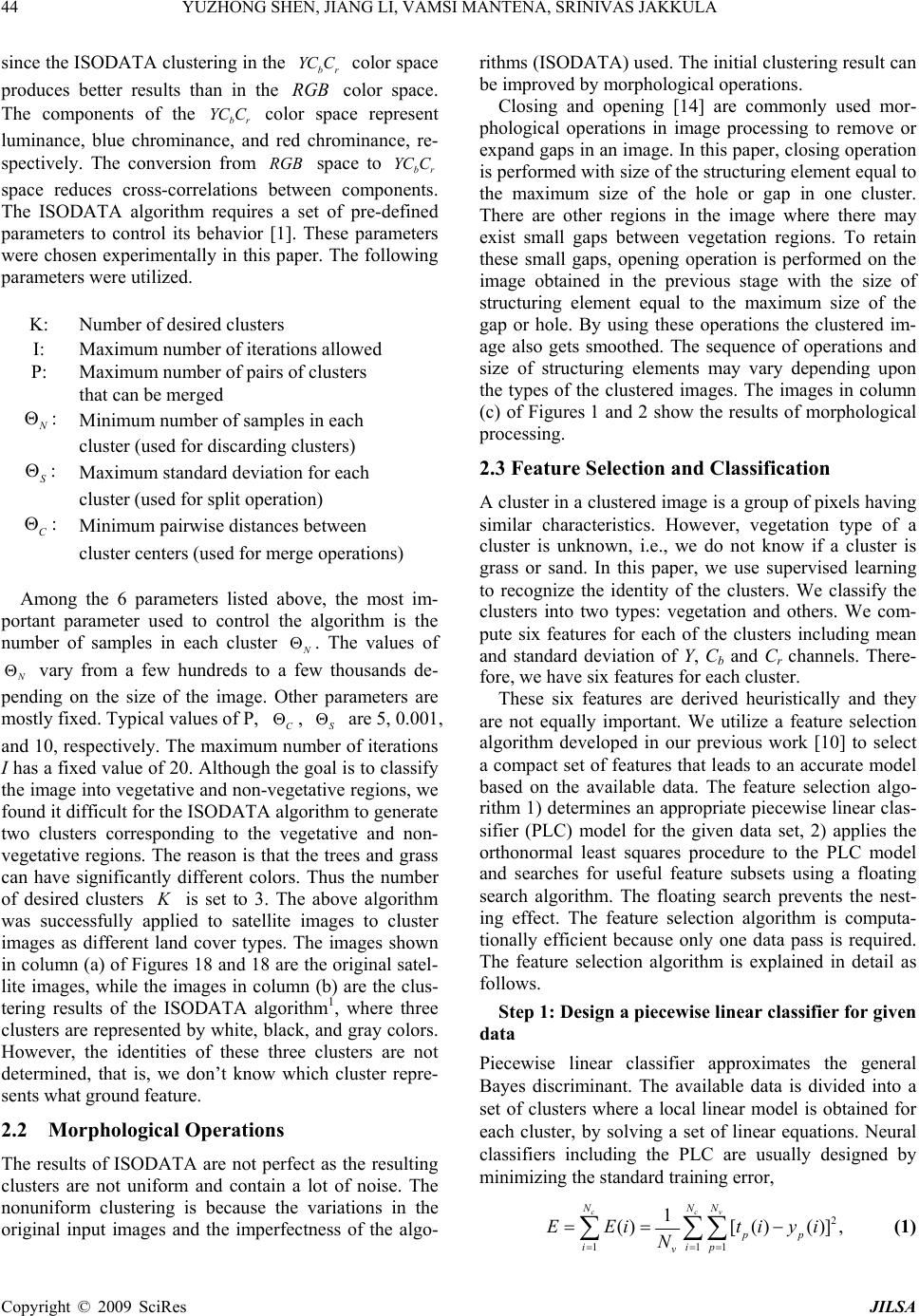

44 YUZHONG SHEN, JIANG LI, VAMSI MANTENA, SRINIVAS JAKKULA
since the ISODATA clustering in the color space
produces better results than in the color space.
The components of the color space represent
luminance, blue chrominance, and red chrominance, re-
spectively. The conversion from
br
YC C
RGB
br
YC C
R
GB
N


e
space to
space reduces cross-correlations between components.
The ISODATA algorithm requires a set of pre-defined
parameters to control its behavior [1]. These parameters
were chosen experimentally in this paper. The following
parameters were utilized.
br
YC C
K: Number of desired clusters
I: Maximum number of iterations allowed
P: Maximum number of pairs of clusters
that can be merged
N
: Minimum number of samples in each
cluster (used for discarding cl ust e rs)
S
: Maximum standard deviation for eac h
cluster (used for split operation)
C
: Minimum pairwi se di st ances bet ween
cluster centers (used for merge operations)
Among the 6 parameters listed above, the most im-
portant parameter used to control the algorithm is the
number of samples in each cluster . The values of
vary from a few hundreds to a few thousands de-
pending on the size of the image. Other parameters are
mostly fixed. Typical values of P, C , S 5, 0.001,
and 10, respectively. The maximum number of iterations
I has a fixed value of 20. Although the goal is to classify
the image into vegetativ e and non-vegetative region s, we
found it difficult for the ISODATA algorithm to generate
two clusters corresponding to the vegetative and non-
vegetative regions. The reason is that the trees and grass
can have significantly different colors. Thus the number
of desired clusters K is set to 3. Thabove algorithm
was successfully applied to satellite images to cluster
images as different land cover types. The images shown
in column (a) of Figures 18 and 18 are the origin al satel-
lite images, while the images in column (b) are the clus-
tering results of the ISODATA algorithm1, where three
clusters are represented by white, black, and gray colors.
However, the identities of these three clusters are not
determined, that is, we don’t know which cluster repre-
sents what ground feature.
N

are
2.2 Morphological Operations
The results of ISODATA are not perfect as the resulting
clusters are not uniform and contain a lot of noise. The
nonuniform clustering is because the variations in the
original input images and the imperfectness of the algo-
rithms (ISODATA) used. The initial clustering result can
be improved by morphological operations.
Closing and opening [14] are commonly used mor-
phological operations in image processing to remove or
expand gaps in an image. In this paper, closing operation
is performed with size of the structuring element equal to
the maximum size of the hole or gap in one cluster.
There are other regions in the image where there may
exist small gaps between vegetation regions. To retain
these small gaps, opening operation is performed on the
image obtained in the previous stage with the size of
structuring element equal to the maximum size of the
gap or hole. By using these operations the clustered im-
age also gets smoothed. The sequence of operations and
size of structuring elements may vary depending upon
the types of the clustered images. The images in column
(c) of Figures 1 and 2 show the results of morphological
processing.
2.3 Feature Selection and Classification
A cluster in a clustered image is a group of pixels having
similar characteristics. However, vegetation type of a
cluster is unknown, i.e., we do not know if a cluster is
grass or sand. In this paper, we use supervised learning
to recognize the identity of the clusters. We classify the
clusters into two types: vegetation and others. We com-
pute six features for each of the clusters including mean
and standard deviation of Y, Cb and Cr channels. There-
fore, we have six features for each cluster.
These six features are derived heuristically and they
are not equally important. We utilize a feature selection
algorithm developed in our previous work [10] to select
a compact set of features that leads to an accurate model
based on the available data. The feature selection algo-
rithm 1) determines an appropriate piecewise linear clas-
sifier (PLC) model for the given data set, 2) applies the
orthonormal least squares procedure to the PLC model
and searches for useful feature subsets using a floating
search algorithm. The floating search prevents the nest-
ing effect. The feature selection algorithm is computa-
tionally efficient because only one data pass is required.
The feature selection algorithm is explained in detail as
follows.
Step 1: Design a piecewise linear classifier for given
data
Piecewise linear classifier approximates the general
Bayes discriminant. The available data is divided into a
set of clusters where a local linear model is obtained for
each cluster, by solving a set of linear equations. Neural
classifiers including the PLC are usually designed by
minimizing the standard training error,
2
111
1
()[ ()()]
ccv
NNN
pp
iip
v
EEi tiyi
N



  (1)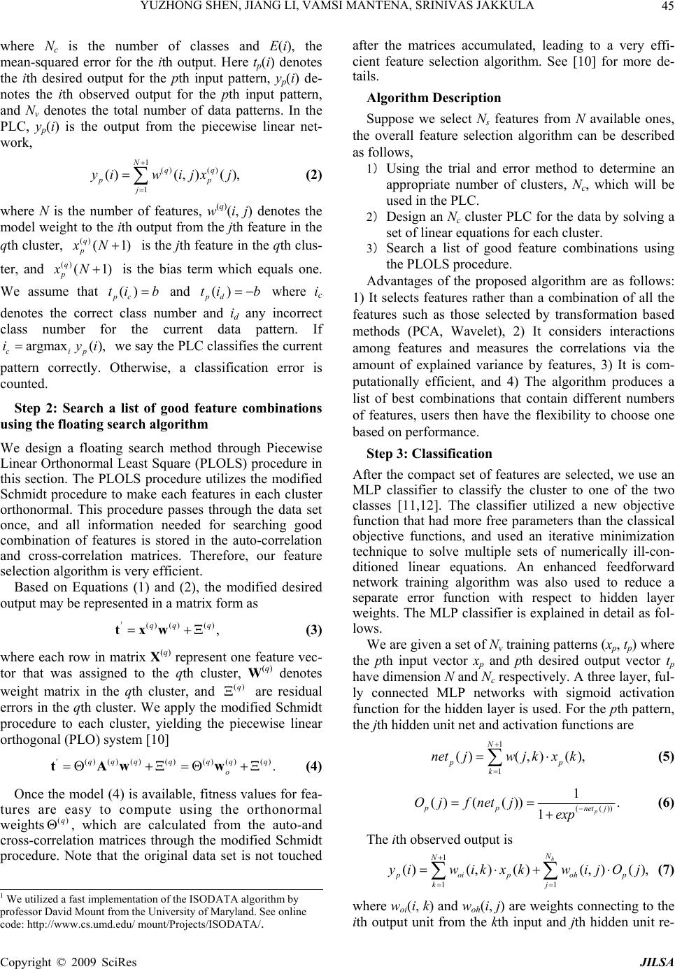

YUZHONG SHEN, JIANG LI, VAMSI MANTENA, SRINIVAS JAKKULA 45
p

)

p
where Nc is the number of classes and E(i), the
mean-squared error for the ith output. Here tp(i) denotes
the ith desired output for the pth input pattern, yp(i) de-
notes the ith observed output for the pth input pattern,
and Nv denotes the total number of data patterns. In the
PLC, yp(i) is the output from the piecewise linear net-
work,
1() ()
1
()()( )
Nqq
p
j
yiw ijxj



 (2)
where N is the number of features, w(q)(i, j) denotes the
model weight to the ith output from the jth feature in the
qth cluster, is the jth feature in the qth clus-
ter, and is the bias term which equals one.
We assume that and where ic
denotes the correct class number and id any incorrect
class number for the current data pattern. If
we say the PLC classifies the current
pattern correctly. Otherwise, a classification error is
counted.
()
(1
q
p
xN
()
(1)
q
xN
()
pc
ti
( )
ip
yi
p
max
b

()
pd
ti b
arg
c
i
Step 2: Search a list of good feature combinations
using the floating search algorithm
We design a floating search method through Piecewise
Linear Orthonormal Least Square (PLOLS) procedure in
this section. The PLOLS procedure utilizes the modified
Schmidt procedure to make each features in each cluster
orthonormal. This procedure passes through the data set
once, and all information needed for searching good
combination of features is stored in the auto-correlation
and cross-correlation matrices. Therefore, our feature
selection algorithm is very efficient.
Based on Equations (1) and (2), the modified desired
output may be represented in a matrix form as
() ()()qqq
txw
＇ (3)
where each row in matrix X(q) represent one feature vec-
tor that was assigned to the qth cluster, W(q) denotes
weight matrix in the qth cluster, and are residual
errors in the qth cluster. We apply the modified Schmidt
procedure to each cluster, yielding the piecewise linear
orthogonal ( PLO) system [10]
()q

() ()()()()()()qqq qqq q
o
 tAww (4)
Once the model (4) is available, fitness values for fea-
tures are easy to compute using the orthonormal
weights , which are calculated from the auto-and
cross-correlation matrices through the modified Schmidt
procedure. Note that the original data set is not touched
()q

after the matrices accumulated, leading to a very effi-
cient feature selection algorithm. See [10] for more de-
tails.
Algorithm Description
Suppose we select Ns features from N available ones,
the overall feature selection algorithm can be described
as follows,
1） Using the trial and error method to determine an
appropriate number of clusters, Nc, which will be
used in the PLC.
2） Design an Nc clus ter PLC for the data by solving a
set of linear equations for each cluster.
3） Search a list of good feature combinations using
the PLOLS procedure.
Advantages of the proposed algorithm are as follows:
1) It selects features rather than a combination of all the
features such as those selected by transformation based
methods (PCA, Wavelet), 2) It considers interactions
among features and measures the correlations via the
amount of explained variance by features, 3) It is com-
putationally efficient, and 4) The algorithm produces a
list of best combinations that contain different numbers
of features, users then have the flexibility to choose one
based on performance.
Step 3: Classification
After the compact set of features are selected, we use an
MLP classifier to classify the cluster to one of the two
classes [11,12]. The classifier utilized a new objective
function that had more free parameters than the classical
objective functions, and used an iterative minimization
technique to solve multiple sets of numerically ill-con-
ditioned linear equations. An enhanced feedforward
network training algorithm was also used to reduce a
separate error function with respect to hidden layer
weights. The MLP classifier is explained in detail as fol-
lows.
We are given a set of Nv training patterns (xp, tp) wher e
the pth input vector xp and pth desired output vector tp
have dimension N and Nc respectively. A three layer, ful-
ly connected MLP networks with sigmoid activation
function for the hidden layer is used. For the pth pattern,
the jth hidden unit net and activation functions are
1
1
()( )()
N
p
k
netjwj kxk



 
 (5)
(())
1
()(()) 1p
pp net j
Oj fnetjexp 


 (6)
The ith observed output is
1
11
()()( )()( )
h
N
N
poipohp
kj
yiwik xkwijO j



 

(7)
1 We utilized a fast implementation of the ISODATA algorithm by
p
rofessor David Mount from the University of Maryland. See online
code: http://www.cs.umd.edu/ mount/Projects/ISODATA/. where woi(i, k) and woh(i, j) are weights connecting to the
ith output unit from the kth input and jth hidden unit re-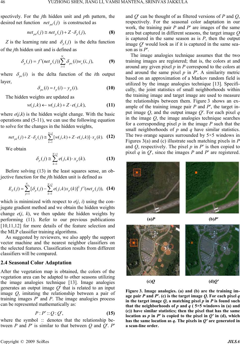

46 YUZHONG SHEN, JIANG LI, VAMSI MANTENA, SRINIVAS JAKKULA
spectively. For the jth hidden unit and pth pattern, the
desired net fun c ti on is constructed as
()
pd
net j
() ()()
pd pp
netjnet jZj

 (8)
Z is the learning rate and ()
pj

is the delta function
of the jth hidden unit and is defined as
1
()(())() ()
c
N
pppoo
i
jfnetj iwij 




(9)
where ()
po i

is the delta function of the ith output
layer, () ()()
po pp
itiyi


p

p


(10)
The hidden weights are updat ed as
() ()()wjkwjkZ ejk  (11)
where e(j,k) is the hidden weight change. With the basic
operations and (5-11), we can use the following equation
to solve for the changes in the hidden weights,
1
1
()()[( )()]()
N
pd pp
k
netjZjwj kZejkxk 


 
 (12)
We obtain
1
1
()()()
N
p
k
jejkxk 



 (13)
Before solving (13) in the least squares sense, an ob-
jective function for the jth hidden unit is defined as
12
11
( )[( )()()](( ))
v
NN
pp
pk
Ejjejkxk fnetj






 (14)
which is minimized with respect to e(j, i) using the con-
jugate gradient method and we obtain the hidden weights
change e(j, k), we then update the hidden weights by
performing (11). Refer to our previous publications
[10,11,12] for more details of the feature selection and
the MLP classifier training algorithms.
As suggested by reviewers, we also apply the support
vector machine and the nearest neighbor classifiers on
the selected features. Classification results from different
classifiers will be compared.
2.4 Seasonal Color Adaptation
After the vegetation map is obtained, the colors of the
vegetation area can be adapted to other seasons utilizing
the image analogies technique [13]. Image analogies
generates an output image Q′ that is related to an input
image Q, imitating the relationship between a pair of
training images P′ and P. The image analogies process
can be represented mathematically as:
PP QQ

 (15)
where the symbol denotes that the relationship be-
tween P and P′ is similar to that between Q and Q′. P′
and Q′ can be thought of as filtered versions of P and Q,
respectively. For the seasonal color adaptation in our
work, the training pair P and P′ are images of the same
area but captured in different seasons, the target image Q
is captured in the same season as is P, then the output
image Q′ would look as if it is captured in the same sea-
son as is P′.

The image analogies technique assumes that the two
training images are registered; that is, the colors at and
around any g iven pixel p in P correspond to the colors at
and around the same pixel p in P′. A similarity metric
based on an approximation of a Markov random field is
utilized by the image analogies technique [13]. Specifi-
cally, the joint statistics of small neighborhoods within
the training image and target image are used to measure
the relationships between them. Figure 3 shows an ex-
ample of the training image pair P and P′, the target in-
put image Q, and the output image Q′. For each pixel q
in the image Q, the image analogies technique searches
for a corresponding pixel p in the image P such that the
small neighborhoods of p and q have similar statistics.
The two orange squares surrounded by 5×5 windows in
Figures 3(a) and (c) illustrate such matching pixels in P
and Q, respectively. The pixel p in P′ is then copied to
pixel q in Q′, since the images P and P′ are registered.
(a)P (b)P′
(c)Q (d)Q′
Figure 3. Image analogies. (a) and (b) are the training im-
age pair P and P′. (c) is the target image Q. For each pixel q
in the target image Q, a matching pixel p in P is found such
that the neighborhoods of p and q ( 5×5 windows in (a) and
(c)) have similar statistics; then the pixel that has the same
location as p in P′ is copied to the pixel in Q′ in (d), which
has the same location as q. The pixels in Q′ are generated in
a scan-line order.

YUZHONG SHEN, JIANG LI, VAMSI MANTENA, SRINIVAS JAKKULA
47
That is, the pixel at the position labeled by the orange
square in Figure 3(b) is copied to the pixel at the position
labeled by the orange square in Figure 3(d). The pixels in
Q are processed in a scan-line order; thus the pixels in Q′
are generated in the same order.
The joint statistics of a small neighborhood centered at
a pixel are concatenation of the feature vectors of all the
pixels in the neighborhood. The feature vector of each
pixel can consist of RGB color components, luminance,
various filter responses, etc. In this work, only RGB col-
or components are included in the feature vector. The
efficient implementation of image analogies technique
makes uses of multi-scale representation and fast neigh-
borhood search methods [13]. The multi-scale represen-
tation first constructs Gaussian pyramids of images P, P′,
and Q with I levels; the synthesis then proceeds from
coarsest to finest resolution, computing a multi-scale
representation of Q′, one level at a time. The pseudocode
of the algorithm [13] is shown below.
BuildImageAnalogy(P, P′, Q)
Construct Gaussian py ramids for P, P′, Q
Compute features for P, P′, Q
for each level i, do:
for each pixel q

Q′ in scan-line order,
do:
P Match
()PP QQ iq


() ()
ii
Qq Pp


Return
I
Q
Q′ I has the finest resolution in the Gaussian pyramid
and it is the final output. The Match() function in the
pseudocode uses fast neighborhood search algorithms,
including the approximate-nearest-neighbor-search [15,
16] and coherence search [17].
As noted in their original work [13], although image
analogies are an effective image synthesis method, it is
not perfect. This can be clearly seen in the example out-
put image Q′ shown in Figure 3(d). The original target
image Q (Figure 3(c)) has some ground objects with
brown colors, but these objects’ colors are changed to
gray in Q′. This is an undesired effect since these ground
objects don’t change their colors in different seasons. To
restrict color changes to vegetative areas only, the vege-
tation map generated in the previous section is utilized.
The vegetation map of Q is shown in Figure 4(a). Utiliz-
ing this vegetation map, non-vegetative regions in Q are
copied back to Q′ to form the final image shown in Fig-
ure 4(b). Our current implementation utilized the code
from [18]. Our future implementation will utilize the
vegetation map in the neighborhood search process, i.e.,
the search is restricted to the vegetative areas of P and Q
only. This will certainly improve the output image qual-
ity since the probability of erroneous neighborhood
match is greatly reduced. The computational time will
also be significantly reduced.
3. Results and Discussion
The results of ISODATA clustering, morphological op-
erations, and classification are shown in columns (b), (c),
and (d) in Figures 1 and 2. To study the effectiveness of
the ISODATA algorithm, we have applied it to the 120
satellite images. A total of 120 satellite images have been
utilized in this study. We computed the six features for
each of the clusters and assigned one class type (vegeta-
tion or non-vegetation) to each of the clusters. The fea-
ture selection algorithm selected three of the features
(means of the Y and Cb channels and standard deviation
of the Cb Channel) and the other three features turned out
to be not useful. To test if a classifier can automatically
identify vegetation type, we used the 5-fold cross-vali-
dation method on the 120 images using three different
classifiers: the MLP classifier described previously, the
support vector machine (SVM) and the k-nearest
neighbor (k-NN) classifier. The MLP has 3 inputs, 1
hidden unit and 2 outputs, and the classifier was trained
by the method described in Subsection 2.3.
Classification results are listed in Table 1. It is clear t-
hat the MLP classifier achieved the best classification a-
ccuracy, 96%, which is slightly better than that of the 1-
NN classifier. The SVM classifier i s the worst in terms of
(a) (b)
Figure 4. (a) Vegetation map of Figure 3(c). (b) Final sea-
sonal color adaptation of Figure 3(c) based on the training
pair in Figure 3(a) and (b).
Table 1. Classification results by three different classifiers.
AlgorithmMLPSVM 1-NN 3-NN 5-NN
Accuracy%96 91.6 94.5 93.6 92.5

48 YUZHONG SHEN, JIANG LI, VAMSI MANTENA, SRINIVAS JAKKULA
(a) (b) (c) (d)
(a) (b) (c) (d)
(a) (b) (c) (d)
(a) (b) (c) (d)
(a) (b) (c) (d)
Figure 1. (a) Initial satellite images, (b) Results of ISODATA clustering, (c) Results of morphological operations. Three clus-
ters are generated, represented by white, black, and gray colors, respectively. However, the identities of the clusters are un-
known, (d) Results of classification. Two classes are generated for non-vegetative and vegetative regions, represented by
white and black masks, respec tively .

49 YUZHONG SHEN, JIANG LI, VAMSI MANTENA, SRINIVAS JAKKULA
(a) (b) (c) (d)
(a) (b) (c) (d)
(a) (b) (c) (d)
(a) (b) (c) (d)
(a) (b) (c) (d)
Figure 2. (a) Initial satellite images. (b) Results of ISODATA clustering. (c) Results of morphological operations. Three clus-
ters are generated, represented by white, black, and gray colors, respectively. However, the identities of the clusters are un-
known. (d) Results of classification. Two classes are generated for non-vegetative and vegetative regions, represented by
white and black masks, respec tively .

50 YUZHONG SHEN, JIANG LI, VAMSI MANTENA, SRINIVAS JAKKULA
(a) (b) (c) (d)
Figure 5. Brown dow n effe ct simulation. (a) and (c ) are input targe t images, while (b) and (d) are output images ge nerated by
the proposed method
(a) (b) (c) (d)
(e) (f) (g) (h)
Figure 6. Green up effect simulation. (a), (c), (e), and (g) are input target images, while (b), (d), (f), and (h) are output images
generated by the proposed algorithm.
accuracy. Based on the results, we can reasonably draw
the conclusion that it is possible to automatically identify
vegetation from other land covers. The MLP classifier
can discriminate the two types with an accuracy of up to
96% in the cross-validation.
Vegetation changes colors due to a number of chemi-
cal, physical, and biological processes that occur in dif-
ferent seasons. It is especially worth to note two phe-
nomena, namely, green up and brown down [1]. In
spring, leaves emerge and flourish and vegetative growth
is rapid, resulting in a greenish appearance, known as
green up. From mid-summer to late summer, plant tis-
sues mature, dry, and are harvested, resulting in a
brownish appearance, referred to as brown down. There
are some other seasonal color changes as well. The im-
ages in Figure 5 simulate the brown down effects. Im-
ages in Figures 5(a) and (c) are input images, while im-
ages in Figures 5(b) and (d) are output images produced
by the proposed method. The images in Figure 6 simu-
late the green up effects. Figures 6(a), (b), (c), and (d)
show the input images, while Figures 6 (e), (f ), (g) , an d (h )
are the output images generated by the proposed method.
These results illustrated the effectiveness of the proposed
method. These results illustrated the effectiveness of the
proposed method. In our current implementation, the
vegetation map only contains vegetative areas (and
therefore non-vegetative areas). To obtain even better
results, the vegetation map needs to be refined, that is, it
should indicate different types of vegetation, such as
trees and grass. Currently the vegetation maps are gener-

51 YUZHONG SHEN, JIANG LI, VAMSI MANTENA, SRINIVAS JAKKULA
ated from satellite images in the visible wavelength band.
In order to obtain better vegetation maps or feature maps,
images from other sources should also be used, such as
infrared images in vari ou s wavelengths.
4. Conclusions
This paper proposed a novel method that alters vegeta-
tion colors in satellite images to simulate seasonal
changes. The proposed method first generates a vegeta-
tion map for pixels corresponding to vegetative areas in
satellite images, using ISODATA clustering and vegeta-
tion classification. It then generates seasonal color adap-
tations of a target input image using an image analogies
technique. The vegetation map ensures that only the col-
ors of vegetative areas are altered. The proposed method
can be used in high performance flight simulations and
other applications.
REFERENCES
[1] J. B. Campbell, “Introduction to remote sensing,” The
Guilford Press, 4th Edition, 2007.
[2] J. P. Wayman, R. H. Wynne, J. A. Scrivani, and G. A.
Burns, “Landsat TM-based forest area estimation using
iterative guided spectral class rejection,” Photogrammet-
ric Engineering and Remote Sensing, Vol. 67, pp. 1155–
1166, 2001.
[3] H. Almuallin and T. G. Dietterich, “Learning with many
irrelevant features,” in Proceedings of AAAI-91, (An-
haim, CA), pp. 547–552, August 1991.
[4] C. Bishop, “Neural networks for pattern recognition,”
New York: Oxford University Press, 1995.
[5] I. V. Tetko, A. E. P. Villa, and D. J. Livingstone, “Neural
network studies. 2: Variable selection,” Journal of Chem-
istry Information and Computer Science, Vol. 36, No. 4,
pp. 794–803, 1996.
[6] K. Kira and L. A. Rendell, “The feature selection prob-
lem: traditional methods and a new algorithm,” in Pro-
ceedings of AAAI-92, (San Jose, CA), pp. 122–126, 1992.
[7] R. Kohavi and G. John, “Wrappers for feature subset
selection,” Artificial Intelligence, Vol. 97, No. 1-2, pp.
273–324, 1997.
[8] J. R. Quinlan, “C4.5: Programs for machine learning,”
San Mateo, California, Morgan Kaufmann, 1993.
[9] L. Breiman, J. Friedman, R. Olshen, and C. Stone,
“CART: Classification and regression trees,” CBelmont,
California, Wadsworth, 1983.
[10] J. Li, M. T. Manry, P. L. Narasimha, and C. Yu, “Feat ure
selection using a piecewise linear network,” IEEE Trans-
actions on Neural Network, Vol. 17, No. 5, pp. 1101–
1105, 2006.
[11] J. Li, M. T. Manry, L. M. Liu, C. Yu, and J. Wei, “Itera-
tive improvement of neural classifiers,” Proceedings of
the Seventeenth International Conference of the Florida
AI Research Society, May 2004.
[12] R. G. Gore, J. Li, M. T. Manry, L. M. Liu, and C. Yu,
“Iterative design of neural network classifiers through re-
gression,” Special Issue of International Journal on Arti-
ficial Intelligence Tools, Vol. 14, No. 1-2, pp. 281–302,
2005.
[13] A. Hertzmann, C. E. Jacobs, N. Oliver, B. Curless, and D.
H. Salesin, “Image analogies,” in the Proceedings of
SIGGRAPH Conference, pp. 327–340, 2001.
[14] S. Chen and R. M. Haralick, “Recursive erosion, dilation,
opening, and closing transforms,” IEEE Transactions on
Image Processing, Vol. 4, No. 3, 1995.
[15] S. Arya, D. M. Mount, N. S. Netanyahu, R. Silverman,
and A. Y. Wu, “An optimal algorithm for approximate
nearest neighbor searching in fixed dimensions,” Journal
of the ACM, pp. 891–923, 1998.
[16] L. Y. Wei and M. Levoy, “Fast texture synthesis using
tree-structured vector quantization,” Proceedings of
SIGGRAPH Conference, pp. 479–488, July 2000.
[17] M. Ashikhmin, “Synthesizing natural textures,” in ACM
Symposium on Interactive 3D Graphics, pp. 217–226,
March 2001.
[18] A. Hertzmann and C. Jacobs, 2001. http://mrl.nyu.edu/
projects/imageanalogies/lf/.