J. Intelligent Learning Systems & Applications, 2009, 1, 28-41
Published Online November 2009 in SciRes (www.SciRP.org/journal/jilsa)
Control Task for Reinforcement Learning with Known
Optimal Solution for Discrete and Continuous Actions
Michael C. RÖTTGER1, Andreas W. LIEHR2
Service-Group Scientific Information Processing, Freiburg Materials Research Center, Freiburg, Germany.
Received November 10th; 2008; revised January 29th, 2009; accepted January 30th, 2009.
ABSTRACT
The overall research in Reinforcement Learning (RL) concentrates on discrete sets of actions, but for certain real-world
problems it is important to have methods which are able to find good strategies using actions drawn from continuous
sets. This paper describes a simple control task called direction finder and its known optimal solution for both discrete
and continuous actions. It allows for comparison of RL solution methods based on their value functions. In order to
solve the control task for continuous actions, a simple idea for generalising them by means of feature vectors is
presented. The resulting algorithm is applied using different choices of feature calculations. For comparing their
performance a simple measure is introduced.
Keywords: comparison, continuous actions, example problem, reinforcement learning, performance
1. Introduction
In Reinforcement Learning (RL), one solves optimal
control problems without knowledge of the underlying
system’s dynamics on the basis of the following perspec-
tive: An agent which is aware of the current state of its
environment, decides in favour of a particular action.
The performance of the action results in a change of the
agent’s environment. The agent notices the new state,
receives a reward, and decides again. This process is
repeated over and over and may be terminated by reach-
ing a terminal state. In the course of time the agent learns
from its experience by developing a strategy which
maximises its estimated total reward.
There are various RL methods for searching optimal
policies. For testing, many authors refer to standard con-
trol tasks in order to enable comparability; others define
their own test-beds or use a specific real-world problem
they want to solve. Popular control tasks used for refer-
ence are e.g. the mountain car problem [1,2,3], the in-
verted pendulum problem [4], the cart-pole swing-up
task [5,6,7] and the acrobot [2,8,9].
In most papers, algorithms are compared by their ef-
fectiveness in terms of maximum total rewards of the
policies found or the number of learning cycles, e.g.
episodes, needed to find a policy with an acceptable
quality. Sometimes the complexity of the algorithms is
also taken into account, because a fast or simple method
is more likely to be usable in practice than a very good
but slow or complicated one. All these criteria allow for
some kind of black-box testing and can give a good es-
timation whether an algorithm is suitable for a certain
task compared to other RL approaches. However, they
are not very good at giving a hint where to search for
causes why an algorithm cannot compete with others or
why, contrary to expectations, no solution is found. The
possible reasons for such kinds of failure are manifold,
starting from bad concepts to erroneous implementa-
tions.
Many ideas in RL are based on representing the
agent’s knowledge by value functions, so their compari-
son among several runs with different calculation
schemes or with known optimal solutions gives more
insight into the learning process and supports systematic
improvements of concepts or implementations.
One control task suitable for this purpose is the double
integrator (e.g. [10]), which has an analytically known
optimal solution for a bounded continuous control vari-
able (the applied force) and the corresponding
state-value function V(s) can be calculated. Since this
produces a bang-bang-like result, the solution for a con-
tinuous action variable does not differ from a dis-
crete-valued control.
In this paper, we present a simple control task, which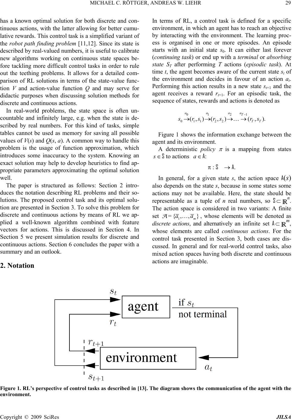

MICHAEL C. RÖTTGER, ANDREAS W. LIEHR29
has a known optimal solution for both discrete and con-
tinuous actions, with the latter allowing for better cumu-
lative rewards. This control task is a simplified variant of
the robot path finding problem [11,12]. Since its state is
described by real-valued numbers, it is useful to calibrate
new algorithms working on continuous state spaces be-
fore tackling more difficult control tasks in order to rule
out the teething problems. It allows for a detailed com-
parison of RL solutions in terms of the state-value func-
tion V and action-value function Q and may serve for
didactic purposes when discussing solution methods for
discrete and continuous actions.
In real-world problems, the state space is often un-
countable and infinitely large, e.g. when the state is de-
scribed by real numbers. For this kind of tasks, simple
tables cannot be used as memory for saving all possible
values of V(s) and Q(s, a). A common way to handle this
problem is the usage of function approximation, which
introduces some inaccuracy to the system. Knowing an
exact solution may help to develop heuristics to find ap-
propriate parameters approximating the optimal solution
well.
The paper is structured as follows: Section 2 intro-
duces the notation describing RL problems and their so-
lutions. The proposed control task and its optimal solu-
tion are presented in Section 3. To solve this problem for
discrete and continuous actions by means of RL we ap-
plied a well-known algorithm combined with feature
vectors for actions. This is discussed in Section 4. In
Section 5 we present simulation results for discrete and
continuous actions. Section 6 concludes the paper with a
summary and an outlook.
2. Notation
In terms of RL, a control task is defined for a specific
environment, in which an agent has to reach an objective
by interacting with the environment. The learning proc-
ess is organised in one or more episodes. An episode
starts with an initial state s0. It can either last forever
(continuing task) or end up with a terminal or absorbing
state ST after performing T actions (episodic task). At
time t, the agent becomes aware of the current state st of
the environment and decides in favour of an action at.
Performing this action results in a new state st+1 and the
agent receives a reward rt+1. For an episodic task, the
sequence of states, rewards and actions is denoted as
0121
011 22
(,)(,)( ,).
aaaa
T
TT
s
rsrsr s

 
Figure 1 shows the information exchange between the
agent and its environment.
A deterministic policy
 is a mapping from states
s

S to actions a

A:
 : S  A.
In general, for a given state s, the action space A(s)
also depends on the state s, because in some states some
actions may not be available. Here, the state should be
representable as a tuple of n real numbers, so Sn.
The action space is considered in two variants: A finite
set 1 ={ ,,}
m
aa, whose elements will be denoted as
discrete actions, and alternatively an infinite set Am,
whose elements are called continuous actions. For the
control task presented in Section 3, both cases are dis-
cussed. In general and for real-world control tasks, also
mixed action spaces having both discrete and continuous
actions are imaginable.
Figure 1. RL’s perspective of control tasks as described in [13]. The diagram shows the communication of the agent with the
environment.

30 MICHAEL C. RÖTTGER, ANDREAS W. LIEHR
In order to handle episodic and continuing tasks with
the same definitions for value functions, we follow the
notation of [13]: Episodic tasks with terminal state sT can
be treated as continuing tasks remaining at the absorbing
state without any additional reward: sT+k≡sT and rT+k≡0
for .

=1,2,3,k
Using this notion, for all states sS, the state-value
function
1
=0
()= =
k
tk t
k
VsErs s








 (1)
concerning a given policy π holds the information, which
total discounted reward can be expected when starting in
state s and following the policy π. The quantity [0,1]


is called discount factor. For <1

the agent is myopic
to a certain degree, which is useful to rank earlier re-
wards higher than latter ones or to limit the cumulative
reward if , i.e. no absorbing state is reached.
=T
In analogy to the value of a given state, one can also
assign a value to a pair (s, a) of state
s
S and action
A(s). The action-value function a
k1
k0
(, )=,
k
tt t
QsaErs sa a












(2)
concerning a policy π is the estimated discounted cumu-
lative reward of an agent in state s, which decides to per-
form the action a and then follows π.
For the deterministic episodic control task proposed in
this paper we have chosen =1

, so the Equations (1)
and (2) simply reduce to finite sums of rewards.
In order to maximise the agent’s estimated total re-
ward, it is useful to define an ordering relation for poli-
cies: A policy π is “better than” a policy π', if
:()()VsV ss




  S. (3)
An optimal policy complies with


 (4)
and is associated with the optimal value functions V
* and
Q* , which are unique for all possible optimal policies:
*(,):=(, ),QsaQ sa 
 (5)
**
():=()=(,).
max
a
VsV sQsa

 (6)
Given the optimal action value function Q* and a current
state s, an optimal action a* can be found by evaluating
*
()=argmax(, ).
a
as Qsa
*
(7)
3. The Directing Problem and Its Solution
3.1 The Control Task
The directing problem is a simplified version of the path
finding problem [11,12] without any obstacles. The
agent starts somewhere in a rectangular box given by


max max
=(x,y)|0 xx0 yy. S (8)
Its real-valued position s=(x, y) is the current state of
the system.
The objective of the agent is to enter a small rectan-
gular area in the middle of the box (Figure 2). This target
area is a square with centre (cx,cy) and a fixed side length
of 2dT. Each position in the target area, including its
boundary, corresponds to a terminal state.
In order to reach this target area, the agent takes one or
more steps with a constant step size of one. Before each
step, it has to decide, which direction to take. If the
resulting position is outside the box, the state will not be
changed at all. So given the state s = (x, y), the action a =
, and using the abbreviation
(, )=(cos ,sin),xy xy




 (9 )
the next state =( ,)
s
xy


is
max max
(, )if(00),
(, )=(, )otherwise.
xyx xyy
xy xy
 

 

 
(10)
In terms of RL, the choice of is the agent’s action
which is always rewarded with r ≡ -1 regardless of the
resulting position. By setting the discount factor =1

,
the total reward is equal to the negative number of steps
needed to reach the target area.
For the analytical solution and for the simulation re-
sults, xmax = ymax = 5, dT =1
2 and cx = cy= 2.5 have been
chosen.
The optimal solution for this problem, although it is
obvious to a human decision maker, has two special fea-
tures:
 In general, the usage of continuous angles allows
for larger total rewards than using only a subset of
discrete angles and

MICHAEL C. RÖTTGER, ANDREAS W. LIEHR31
Figure 2. The direction finder. The state of the agent is its real-valued position somewhere in the simulation domain. Its
objective is to enter the shaded target area by choosing a direction before each constant-sized step. This choice may be
completely free (continuous actions) or limited to a finite number of four angles (discrete actions). The reward after each step
is -1, so an optimal policy would minimise the total number of steps.
 the state value function V
* and Q* can be expressed
analytically, so intermediate results of reinforce-
ment learning algorithms can be compared to the
optimal solution with arbitrary precision.
In the following, the solutions for discrete and con-
tinuous actions are described.
3.2 Discrete Actions
For a finite set
(11)
of four discrete directions, which can be coded as
3
0,, ,
22








using angles in radians, the state value for
an optimal policy for an arbitrary position (x, y) is given
by
*
discr (, )=(())(()). xy
Vxy hgxhgy   (12)
The symbol denotes the ceiling function, which
returns the smallest integer equal to or greater than a
given number, and the terms and
are abbreviations for

(())
x
hg x(())
y
hgy
()=| |
x
xT
g
xxcd (13)
()=| |
yyT
g
yycd (14)
0for 0
()=zfor 0
z
hz z



 (1 5)
The value of a terminal state is zero, since no step is
needed.
Figure 3 shows a plot of the optimal state-value func-
tion for discrete actions. Due to the limited set of direc-
tions, the agent needs four steps when starting in a corner
of the domain.
3.3 Continuous Actions
If arbitrary angles [0,2 ]


are allowed, i.e. continu-
ous actions, the optimal state value is given by:
22
cont(,) =(())(()). xy
Vxyhgxhgy





 (16)
As for discrete actions, the helper functions defined in
(13), (14), and (15) have been used.
Figure 4 shows a plot of the optimal state-value func-
tion for continuous actions. Contrary to the case of dis-
crete actions, the agent only needs three steps at the most
to enter the target area. Except for the set of possible
directions, the task specification is the same as for dis-
crete actions.

32 MICHAEL C. RÖTTGER, ANDREAS W. LIEHR
Figure 3. Optimal state value function V *(x, y) for four discrete actions → , ↑ , ← and ↓ . Because of 1

 it is equal to the
negative number of steps needed in order to enter the target square in the centre, so V
*(x, y)


4, 3,1,02, . xmax = ymax =
5, dT =1
2 and cx = cy= 2.5.
Figure 4. Optimal state value function V
*(x, y) for continuous actions, i.e. [0, 2[


. The state value is equal to the negative
number of steps needed to enter the target square in the centre, so V
*(x, y)


3, 2,1,0 . xmax = ymax = 5, dT =1
2 and cx = cy=
2.5.

MICHAEL C. RÖTTGER, ANDREAS W. LIEHR33
Figure 5. Action values for all states when choosing direction → (or =0) as first action and following an opti- mal policy
with discrete actions afterwards. The corresponding state value function is depicted in Figure 3. Values rank from −5 to 0.
Figure 6. Action values for all states when choosing direction → (or =0) as first action and following an optimal policy for
continuous actions afterwards. The according state value function is depicted in Figure 4. Values rank from −4 to 0.

34 MICHAEL C. RÖTTGER, ANDREAS W. LIEHR
3.4 Action Values
The problem as defined above is deterministic. With
given and
(, )Vxy
=1

, the evaluation of the corre-
sponding action value function is as simple as calculating
the state value of the subsequent state (x', y') by means of
(9) and (10), except for absorbing states:
Q*(x,y,) (17)
*
0 if(x,y)isterminal,
=( ,) 1otherwise,



Vxy
where the next state (x', y') is defined by (10). Its optimal
state value V *(x', y') is computed through evaluation of
(12) for discrete actions or (16) for continuous actions.
For the direction →, or =0, the action value func-
tion Q* (x, y, →) is depicted in Figure 5 for four discrete
angles (→, ↑, ←,↓ ) and in Figure 6 for continuous an-
gles. Disregarding the target area both plots can be de-
scribed by V
* (s)－1 shifted to the left with a respective
copy of the values for to .
]3,4]x]4,5]x
4. Algorithm for Searching Directions with
Reinforcement Learning
In the following an algorithm is presented which is capa-
ble of solving the direction finder problem for discrete
and continuous actions. It is based on a linear approxi-
mation of the action value function Q and is often
used and well-known for discrete actions. Note, that we
have slightly changed the notation in order to apply ideas
from state generalisation to the generalisation of actions,
which enables us to handle continuous actions.
Q

4.1 Handling of Discrete and Continuous Actions
When searching for a control for tasks with a small finite
number of actions (discrete actions), it is possible to as-
sign an individual approximation function (, )()

a
QsaQs
ble action. When using linear approxima-
tion, this is often implemented by using a fixed feature
vector for every state s independent of an action a and a
separate weight vector θa for every action:
to every possi
a
()=  θ

a
Qs  (s) (18)
For a very large set of possible actions, e.g. if the ac-
tion is described by (dense) real-valued numbers drawn
from an interval (continuous actions), this approach
reaches its limits. In addition, the operation(, )
maxaQsa


becomes very expensive when implemented as brute
force search over all possible actions and can hardly be
performed within a reasonable time.
There are many ideas for dealing with continuous ac-
tions in the context of Reinforcement Learning. Exam-
ples are the wirefitting approach [14], the usage of an
incremental topology preserving map building an aver-
age value from evaluating different discrete actions [15]
and the application of neural networks (e.g. [16]).
To the best of our knowledge, so far no method has
been shaped up as the algorithm of choice; so we want to
contribute another idea which is rather simple and has
been successfully applied to the direction finder problem.
The basic idea, which is more a building block than a
separate method, is not only to use feature vectors for
state generalisation, but also to calculate separate feature
vectors for actions. We combine state and action features
in such a manner that each combination of feature com-
ponents for a state and for an action uses a separate
weight. If one has a combined feature  (s,a), the linear
approximation can be expressed as
(, )=Qsa

θ

 (s,a) (19)
where each weight, a component of θ, refers to a combi-
nation of certain sets of states and actions. This raises the
question how to build a combined feature vector  (s,a).
Here, two possibilities are considered.
Having a state feature and an action fea-
ture , with components
and (20)
(21)
an obvious way of combination would be to simply con-
catenate (CC) them:
(22)
(23)
Concerning linear approximation, this would lead to a
separation in weights for states and actions which is not
suitable for estimating Q(s, a) in general, because the
coupling of states and actions is lost:

MICHAEL C. RÖTTGER, ANDREAS W. LIEHR35
(24)
Alternatively, one can form a matrix product (MP) of
the feature vectors which results in a weight for every
combination of components of the vectors and
building a new feature vector:
(25)
with =1,,, =1,,.
s
a
injn
The resulting matrix has been reshaped to a vector by
concatenating the rows in order to stick with the termi-
nology of a feature vector. This kind of feature assem-
bling has been used for the results in the following sec-
tions. From now on, the tag MP is left out for better
readability.
With this kind of combined feature vector, the known
case of discrete actions with separate weights for each
action can be expressed by means of (19). This is done
by choosing the action’s feature vector as
(26 )
with and
for =i aa and 0 otherwise. This is equivalent to the
usage of binary features with only one feature present,
the latter corresponds to the action a.
For continuous actions, all methods to calculate fea-
ture vectors for states can also be considered to be used
for actions. One has to choose some appropriate way to
generalise every action by a feature vector.
There are several ideas for procedures to compute a
feature vector. One of the most popular is the usage of tile
coding in a Cerebellar Model Articulation Controller
(CMAC) architecture, e.g. successfully applied for con-
tinuous states in [2]. A comparison of radial-based fea-
tures (RBF) with CMAC for function approximation is
given in [17]. In the following, we present different kinds
of state and action features used for the direction finder.
4.2 State Features
One of the simplest feature types are binary features. For
states of the direction finder, we used the square-shaped
areas
(2 7)
for with centres
,=1, ,20ij 
2121
=,. (28)
88
ij
ij
c



S
For binary state features we evaluate
(29 )
Here s denotes the tuple (x, y). Row by row, the com-
ponents of (29) are combined to a feature vector
.
Similarly, for radial-based state features we used
(30)
Again, the components are combined to a feature vec-
tor which is additionally normalised afterwards:
(31)
4.3 Action Features
For the set of discrete actions Equation (26) results in a
binary feature vector
(32)
For continuous actions a, i.e. for arbitrary angles
[0,2 ]


, we use the sixteen components
(33)
with and
=1, ,16l. These compo-
nents decay quite fast and can be regarded as zero when
used at a distance of 2π from the centers of the
Gaussians:
(34)
This is used to build feature vectors accounting for the
periodicity
**
(, , )=(, ,2),QxyQxy

 
which should be met by the approximation (, ,)Qxy

.
In order to approximately achieve this, we combine the
Gaussians as

36 MICHAEL C. RÖTTGER, ANDREAS W. LIEHR
(35)
and define a normalised action feature vector
(36)
which is finally used in (25) as .
Using Equations (34), (35), (25) and (19) it follows that
Feature vectors for continuous angles built like this are
henceforth called cyclic radial-based. In order to have a
second variant of continuous action features at hand, we
directly combine the components defined in (33)
to a feature vector and normalise it in a way equivalent
to (36). These features are denoted with the term ra-
dial-based and are not cyclic.
4.4 Sarsa( λ ) Learning
For the solution of the direction finder control task, the
gradient-descent Sarsa(λ) method has been used in a
similar way as described in [13] for a discrete set of ac-
tions when accumulating traces. The approximation
of Q is calculated on the basis of (19) using (23) for  (s,a)
with features as described in Subsections 4.2 and 4.3.
The simulation started with =0 . There were no
random actions and the step-size parameter
Q

0
tθ

for the
learning process has been held constant at 0.5=

.
Since the gradient of is  (s,a), the update rule can
be summarised as
Q

111
=(,;)(,;
ttttt ttt
rQsaQsa 



θθ)
t
 (s)
=rt+1+ 
tT(
 (st+1,at+1)-(st,at)) (37)
1= ttt

θθδe (38)
et+1=et+  (st+1,at+1) (39)
The vector et holds the eligibility traces and is initial-
ised with zeros for t = 0 like θt. An episode stops when
the agent encounters a terminal state or when 20 steps
are taken.
4.5 Action Selection
Having an approximation (s,a) at hand, one has to
provide a mechanism for selecting actions. For our ex-
periments with the direction finder, we simply use the
greedy selection
Q

()=argmax(, ).
a
s
Qsa 
 (40)
For discrete actions, π(s) can be found by comparing
the action values for all possible actions. For continuous
actions in general, the following issues have to be con-
sidered:
1) standard numerical methods for finding extrema
normally search for a local extremum only,
2) the global maximum could be located at the
boundary of (s), and
3) the search routine operates on an approximation
Q
(s,a) of Q(s,a).
For the results of this paper, the following approach
has been taken: The first and the second issue are faced
by evaluating (, , )Qxy

 at 100 uniformly distributed
actions besides =0 and =2π, taking the best candi-
date in order to start a search for a local maximum. The
latter has been done with a Truncated-Newton method
using a conjugate-gradient (TNC), see [18]. In general,
in the case of multidimensional actions , the problem
of global maxima at the boundary of
a
(s) may be tack-
led by recursively applying the optimisation procedure
on subsets of (s) and fixing the appropriate compo-
nents of a at the boundaries of the subsets. The third is-
sue, the approximation, cannot be compassed, but allows
for some softness in the claim for accuracy, which may
be given as an argument to the numerical search proce-
dure.
5. Simulation Results
In the following, the direction finder is solved by apply-
ing variants of the Sarsa(λ) algorithm, which differ in the
choice of features for states and actions. Each of them is
regarded as a separate algorithm whose effectiveness
concerning the direction finder is expressed by a single
number, the so-called detour coefficient. In order to
achieve this, the total rewards obtained by the agent are
related to the optimal state values V *(s0), where s0 is the
randomly chosen starting state varying from episode to
episode.

MICHAEL C. RÖTTGER, ANDREAS W. LIEHR37
5.1 Detour Coefficient
Let be a set of episodes. We define a measure called
detour coefficient
 () by
(41)
Here, Re is the total (discounted) reward obtained by
the agent in episode e and is the respective initial
state. The quantity |
e
s0
| denotes the number of episodes in
. In our results the ||=1000 last non-trivial episodes
have been taken into account to calculate the detour co-
efficient by means of (41), whereas non-trivial means
that the episodes start with a non-terminal state, so the
agent has to decide for at least one action. For V * one has
to choose from Equations (12) and (16) according to the
kind of actions used.
The smaller  (), the more effective a learning pro-
cedure is to be considered. For the direction finder, the
value of  () can be interpreted as the average number
of additional steps per episode the RL agent needs in
comparison to an omniscient agent. It always holds that
 ( ), because the optimal solution cannot be out-
performed.
0
The detour coefficient depends on the random set of
starting states of the episodes e, therefore we con-
sider  () as an estimator and assign a standard error for
the mean by evaluating
(42)
with .
0
=*()
ee
eVs R
 
For the following results, the set of randomly chosen
starting states is the same for the algorithms compared to
each other.
5.2 Discrete Actions
For discrete actions, we have solved the direction finder
problem for two different settings, with binary state fea-
tures according to (29) and with radial-based state fea-
tures according to (30) and (31). The other parameters
were: 10000 episodes, 0.5=

, 0.3

, max 20T

.
Calculating the detour coefficient (41) for the last 1000
episodes not having a terminal initial state we observe
 ()=0 for binary state features. This means, these epi-
sodes have an optimal outcome. Repeating the simula-
tion with radial-based state features, there were six epi-
sodes of the last 1000 non-trivial episodes which in total
took 12 steps more than needed, so  ( ).
The respective approximation Qx
0.012 0.005
, )(,y


(Qx

after 10000
episodes for radial-based state features is shown in Fig-
ure 7a as image plot which is overlayed by a vector plot
visualising the respective greedy angles. An illustration
of the difference *(, )max
Vxy ,, )y

 for sample
points on a grid is depicted in Figure 7b. Due to (6) such
a plot can give a hint, where the approximation is inac-
curate. Here the discontinuities of V * stand out.
Both kinds of features are suitable in order to find an
approximation from which a good policy can be
deduced, but the binary features perform perfectly in the
given setting, which is not surprising because the state
features are very well adapted to the problem.
Q

5.3 Continuous Actions
For continuous actions, which means [0, 2[

, solu-
tions of the direction finder problem have been obtained
for four different combinations of state and action fea-
tures. The feature vectors have been constructed as de-
scribed in Subsections 4.2 and 4.3. The results are sum-
marized in Table 1.
For all simulations the following configuration has
been used: 0.5=

, 0.3


, maximum episode time
max 20T

, and 20000 episodes. The values of  () and
s

() have been calculated as discussed in Subsection
5.1. Like for binary state features and discrete actions,
the last 1000 non-trivial episodes did not always result in
an optimal total reward, so  ()>0 for every algorithm.
Our conclusion with respect to these results for the given
configuration and control task is:
 Radial-based state features are more effective than
binary state features.
 When using radial-based state features, cyclic ra-
dial-based action features outperform radial-based
features lacking periodicity.
Table 1. Results for continuous actions for different
combinations of state and action features:
bin (binary), rb (radial-based), crb (cyclic radial-based).
state featuresaction features η(ε) sη(ε)
bin rb 0.109 0.011
bin crb 0.115 0.013
rb rb 0.090 0.011
rb crb 0.063 0.009

38 MICHAEL C. RÖTTGER, ANDREAS W. LIEHR
(a)
(b)
Figure 7. Results for learning with discrete actions, calculated by performing 10000 episodes, using radial-based state
features. Possible directions: . For parameters, see Subsection 5.2. For these plots, the value functions and
the policy have been evaluated on 40x40 points on a regular grid in the state space. (a) Discrete greedy actions
φ{,,,}∈
argmax
gφ
φ
=Q(x,
y
,
φ
)
 and their values 
g
Q(x . The angles corresponding to the greedy actions are denoted by
arrowheads. (b) Difference between
, y,
(, )

Vx
φ)
y
and (
maxφQx,y,)

φ
. The largest deviations are at the lines of discontinuity of
(, )

Vx
y
. Compare to Figure 3.

MICHAEL C. RÖTTGER, ANDREAS W. LIEHR39
(a)
(b)
Figure 8. Results for learning with continuous actions, calculated by performing 20000 episodes, using radial- based state
features and cyclic radial-based action features. In principal, all directions are selectable: . For parameters see
Subsection 5.3. Like in Figure 7, for the sampling of a regular grid of 40x40 points has been used. (a)
Continuous greedy actions
[∈φ0,2π[
)(
maxφQx,y,φ
argmax
gφ
φ=Q(x,
y
,φ)
 and their values 
g
Q(x
(, )

Vx
, y,φ). The angles corresponding to the greedy
actions are denoted by arrowheads. (b) Difference between
y
and ()

Qx,y,
maxφ
φ
. The largest deviations are located
near the discontinuities of (,)

Vx
y
. Compare with Figrue 4.

40 MICHAEL C. RÖTTGER, ANDREAS W. LIEHR
Figure 8 illustrates the function ),,(
~
max


yxQ
Vx

*
V
and
its comparison with V*(x, y) for radial-based state fea-
tures and cyclic radial-based action features after 20000
episodes. Monitoring this difference during the learning
process helps to understand where difficulties for the
approximation scheme or the action selection arise. Here,
like for discrete actions, the discontinuities of
stand out. In order to get additional information, one can
add an estimation procedure for resulting in an ap-
proximation , e.g. by using the TD(
(, )y
V


) algorithm
[13,19], which runs independently in parallel to the
learning process. Inspecting the evolution of supports
an assessment about the covering of the state space.
V

6. Conclusions and Outlook
The direction finder is a control task in the domain of
real-valued state spaces which allows choosing either
discrete or continuous actions. For both cases, the opti-
mal value functions and are known analytically
and can be compared with their approximations in detail.
The optimal policy for continuous actions is not
bang-bang-like and generally results in at least as good
or better total rewards than the optimal policy used for
four discrete actions. In general, the application of fine
discretisations of the action space in order to find a con-
tinuous policy is not an option. In the case of the direc-
tion finder, one could think about using
discrete angles because the solution should converge to
the solution for optimal angles, but the mere effort to
find a greedy action increases linearly with the number
of actions. In general, problems with continuous actions
cannot be solved in a satisfying way by simply refining
the methods for discrete actions but require new ideas.
The development of these ideas is supported by evident
control tasks like the direction finder.
*
V* Q
8,16,32, 
Together with a measure like the detour coefficient
(41), the direction finder can serve as a tool for testing
new RL algorithms working on real-valued state spaces
for both discrete and continuous actions allowing for
intermediate comparison of the approximations and
with the known optimal value functions and .
The detour coefficient can also be used in combination
with any other control task for which the optimal state
value function is known.
V

Q
*
V* Q
*
V
In order to solve the control task for continuous ac-
tions, we have introduced feature vectors for actions in
order to approximate . This may serve as a
building block in other Reinforcement Learning algo-
rithms.
(, )Qsa

The proposed algorithm has been applied to the direc-
tion finder control task for discrete and continuous ac-
tions using different combinations of features. In the case
of continuous actions, we are able to infer from the de-
tour coefficient that certain kinds of features are more
suitable than others.
There are many improvements which can be applied to
the search algorithm. So far, when searching for
, the linearity of together with the
knowledge of the feature calculation scheme has not
been taken into account. This may result in faster and
more accurate optimisation. In addition, it would be in-
teresting to use the detour coefficient to compare the
algorithm with completely different approaches for con-
tinuous actions or other kinds of action selection.
argmax(,)
aQsa
Q 
Based on the known optimal solution, a debugging
procedure can be defined, which helps to ensure that the
basic capabilities of a new algorithm are present. As-
suming the existence of an interface which allows
switching between control tasks without changing the
implementation of the algorithm, the implementation can
be debugged with the presented direction finder control
problem whose solution is exactly known in detail.
Such a debugging procedure can be composed of five
subsequent steps:
1) Implement the proposed control task, the direction
finder, along with functions to calculate * V(s) and
*
Q(s,a).
2) Prove the action selection capabilities by applying
it to * Qand compare the outcome of several runs with
*
V(s0).
3) Prove the approximation abilities by “setting” the
current approximation Q
 of the action value function
to * Qas closely as possible, e.g. by using minimal
least- squares.
4) Prove the stability of the algorithm by starting with
the approximation of * Q from the previous step, per-
forming several learning cycles and testing for simi-
larity of *(,) and * V(s).
maxaQsa
5) Prove the convergence of the algorithm by starting
with sparse or no previous knowledge and searching a
“good” approximation Q
(s,a) for *
Q(s,a).
These checks can be evaluated by comparing
maxaQ*(s,a) or with V*(s) or using a meas-
ure like the detour coefficient as defined in (39). If an
max(,)
aQsa


MICHAEL C. RÖTTGER, ANDREAS W. LIEHR41
algorithm fails to pass this procedure, it will probably
fail in more complex control tasks.
The direction finder is an example problem suitable
for the testing of algorithms which are able to work on
two-dimensional continuous state spaces, but there are
more use cases, e.g. with more dimensions of state
and/or action spaces. A collection of similar control
problems with known optimal solutions (e.g. more com-
plex or even simpler tasks) together with a debugging
procedure can comprise a toolset for testing and com-
paring various Reinforcement Learning algorithms and
their configurations respectively.
7. Acknowledgment
We would like to thank Prof. J. Honerkamp for fruitful
discussions and helpful comments.
REFERENCES
[1] J. A. Boyan and A. W. Moore, “Generalization in rein-
forcement learning: Safely approximating the value func-
tion,” in Advances in Neural Information Processing Sys-
tems 7, The MIT Press, pp. 369-376, 1995.
[2] R. S. Sutton, “Generalization in reinforcement learning:
Successful examples using sparse coarse coding,” in Ad-
vances in Neural Information Processing Systems, edited
by David S. Touretzky, Michael C. Mozer, and Michael
E. Hasselmo, The MIT Press, Vol. 8, pp. 1038-1044,
1996.
[3] W. D. Smart and L. P. Kaelbling, “Practical reinforce-
ment learning in continuous spaces,” in ICML’00: Pro-
ceedings of the Seventeenth International Conference on
Machine Learning, Morgan Kaufmann Publishers Inc., pp.
903-910, 2000.
[4] M. G. Lagoudakis, R. Parr, and M. L. Littman, “Least-
squares methods in reinforcement learning for control,”
in Proceedings of Methods and Applications of Artificial
Intelligence: Second Hellenic Conference on AI, SETN
2002, Thessaloniki, Greece, Springer, pp. 752-752, April
11-12, 2002.
[5] K. Doya, “Reinforcement learning in continuous time and
space,” Neural Computation, Vol. 12, pp. 219-245, 2000.
[6] P. Wawrzy ński and A. Pacut, “Model-free off-policy
reinforcement learning in continuous environment,” in
Proceedings of the INNS-IEEE International Joint Con-
ference on Neural Networks, pp. 1091-1096, 2004.
[
7] J. Morimoto and K. Doya, “Robust reinforcement learn-
ing,” Neural Computation, Vol. 17, pp. 335-359, 2005.
[8] G. Boone, “Efficient reinforcement learning: Model-
based acrobot control,” in International Conference on
Robotics and Automation, pp. 229-234, 1997.
[9] X. Xu, D. W. Hu, and X. C. Lu, “Kernel-based least
squares policy iteration for reinforcement learning,”
IEEE Transactions on Neural Networks, Vol. 18, pp.
973-992, 2007.
[10] J. C. Santamaría, R. S. Sutton, and A. Ram, “Experiments
with reinforcement learning in problems with continuous
state and action spaces,” Adaptive Behavior, Vol. 6, pp.
163-217, 1997.
[11] J. D. R. Millán and C. Torras, “A reinforcement connec-
tionist approach to robot path finding in non-maze-like
environments,” Machine Learning, Vol. 8, pp. 363-395,
1992.
[12] T. Fukao, T. Sumitomo, N. Ineyama, and N. Adachi,
“Q-learning based on regularization theory to treat the
continuous states and actions,” in the 1998 IEEE Interna-
tional Joint Conference on Neural Networks Proceedings,
IEEE World Congress on Computational Intelligence,
Vol. 2, pp. 1057-1062, 1998.
[13] R. S. Sutton and A. G. Barto, “Reinforcement learning:
An introduction of adaptive computation and machine
learning,” The MIT Press, March 1998.
[14] L. C. Baird and A. H. Klopf, “Reinforcement learning
with high-dimensional, continuous actions,” Technical
Report, WL-TR-93-1147, Wright-Patterson Air Force
Base Ohio: Wright Laboratory, 1993.
[15] J. D. R. Millán, D. Posenato, and E. Dedieu, “Continu-
ous-action q-learning,” Machine Learning, Vol. 49, pp.
247-265, 2002.
[16] H. Arie, J. Namikawa, T. Ogata, J. Tani, and S. Sugano.
“Reinforcement learning algorithm with CTRNN in con-
tinuous action space,” in Proceedings of Neural Informa-
tion Processing, Part 1, Vol. 4232, pp. 387-396, 2006.
[17] R. M. Kretchmar and C. W. Anderson, “Comparison of
CMACS and radial basis functions for local function ap-
proximators in reinforcement learning,” in International
Conference on Neural Networks, pp. 834-837, 1997.
[18] R. Dembo and T. Steihaug, “Truncated-Newton algo-
rithms for large-scale unconstrained optimization,”
Mathematical Programming, Vol. 26, pp.190-212, 1983.
[19] R. S. Sutton, “Learning to predict by the methods of
temporal differences,” Machine Learning, Vol. 3, pp.
9-44, 1988.