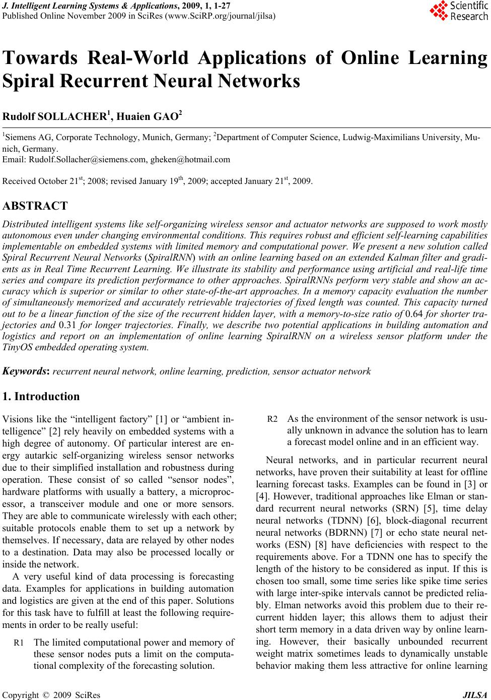J. Intelligent Learning Systems & Applications, 2009, 1, 1-27
Published Online November 2009 in SciRes (www.SciRP.org/journal/jilsa)
Towards Real-World Applications of Online Learning
Spiral Recurrent Neural Networks
Rudolf SOLLACHER1, Huaien GAO2
1Siemens AG, Corporate Technology, Munich, Germany; 2Department of Computer Science, Ludwig-Maximilians University, Mu-
nich, Germany.
Received October 21st; 2008; revised January 19th, 2009; accepted January 21st, 2009.
ABSTRACT
Distributed intelligent systems like self-o rganizing wireless sensor and actuator networks are suppo sed to work mostly
autonomous even und er changing enviro nmenta l conditio ns. This requires ro bust and efficient self-learning capabilities
implemen table on embedded sys tems with limited memory and computational power. We present a new solutio n called
Spiral Recurrent Neural Networks (SpiralRNN) with an online learning based on an extend ed Kalman filter and gradi-
ents as in Real Time Recurrent Learning. We illustrate its stability and performance using artificial and real-life time
series and compare its prediction performance to other approaches. SpiralRNNs perform very stable and show an ac-
curacy which is superior or similar to other state-of-the-art approaches. In a memory capacity evaluation the number
of simultaneously memorized and accurately retrievable trajectories of fixed length was counted. This capacity turned
out to be a linear function of the size of the recurrent hidden layer, with a memory-to-size ratio of 0.64 for shorter tra-
jectories and 0.31 for longer trajectories. Finally, we describe two potential applications in building automation and
logistics and report on an implementation of online learning SpiralRNN on a wireless sensor platform under the
TinyOS embedded operating system.
Keywords: recurrent neural network, online learning, prediction, sensor actuator network
1. Introduction
Visions like the “intelligent factory” [1] or “ambient in-
telligence” [2] rely heavily on embedded systems with a
high degree of autonomy. Of particular interest are en-
ergy autarkic self-organizing wireless sensor networks
due to their simplified installation and robustness during
operation. These consist of so called “sensor nodes”,
hardware platforms with usually a battery, a microproc-
essor, a transceiver module and one or more sensors.
They are able to communicate wirelessly with each other;
suitable protocols enable them to set up a network by
themselves. If necessary, data are relayed by other nodes
to a destination. Data may also be processed locally or
inside the network.
A very useful kind of data processing is forecasting
data. Examples for applications in building automation
and logistics are given at the end of this paper. Solutions
for this task have to fulfill at least the following require-
ments in order to be really useful:
R1 The limited computational power and memory of
these sensor nodes puts a limit on the computa-
tional complexity of the forecasting solution.
R2 As the environmen t of the sensor networ k is usu-
ally unknown in adv ance th e solution has to learn
a forecast model online and in an efficient way.
Neural networks, and in particular recurrent neural
networks, have pro ven their suitability at least for offline
learning forecast tasks. Examples can be found in [3] or
[4]. However, traditional approaches like Elman or stan-
dard recurrent neural networks (SRN) [5], time delay
neural networks (TDNN) [6], block-diagonal recurrent
neural networks (BDRNN) [7] or echo state neural net-
works (ESN) [8] have deficiencies with respect to the
requirements above. For a TDNN one has to specify the
length of the history to be considered as input. If this is
chosen too small, some time series like spike time series
with large inter-spike interv als cannot be predicted relia-
bly. Elman networks avoid this problem due to their re-
current hidden layer; this allows them to adjust their
short term memory in a data driven way by online learn-
ing. However, their basically unbounded recurrent
weight matrix sometimes leads to dynamically unstable
behavior making them less attractive for online learning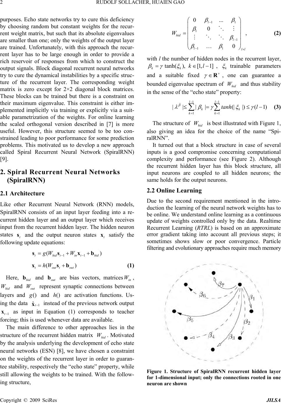

RUDOLF SOLLACHER, HUAIEN GAO
2
purposes. Echo state networks try to cure this deficiency
by choosing random but constant weights for the recur-
rent weight matrix, but such that its ab solute eigenvalues
are smaller than one; only the weights of the outpu t layer
are trained. Unfortunately, with this approach the recur-
rent layer has to be large enough in order to provide a
rich reservoir of responses from which to construct the
output signals. Block diagonal recurrent neural networks
try to cure the dynamical instabilities by a specific struc-
ture of the recurrent layer. The corresponding weight
matrix is zero except for 2×2 diagonal block matrices.
These blocks can be trained but there is a constraint on
their maximum eigenvalue. This constraint is either im-
plemented implicitly via training or explicitly via a suit-
able parametrization of the weights. For online learning
the scaled orthogonal version described in [7] is more
useful. However, this structure seemed to be too con-
strained leading to poor performance for some prediction
problems. This motivated us to develop a new approach
called Spiral Recurrent Neural Network (SpiralRNN)
[9].
2. Spiral Recurrent Neural Networks
(SpiralRNN)
2.1 Architecture
Like other Recurrent Neural Network (RNN) models,
SpiralRNN consists of an input layer feeding into a re-
current hidden layer and an output layer which receives
input from the recurrent hidden layer. The hidden neuron
states t and the output neuron states satisfy the
following u pdate equations:
st x
11
()
thidtinth
gW W

ssxb
id
) (
tout tout
hWxsb (1 )
Here, and are bias vectors, matrices,
and represent synaptic connections between
layers and
hid
b
out
W
out
bin W
hid
W
()
g
and are activation functions. Us-
ing the data instead of the previous network output
as input in Equation (1) corresponds to teacher
forcing; this is used when ever data are available.
()h
1
ˆ xt
1t
x
The main difference to other approaches lies in the
structure of the recurrent hidden matrix . Motivated
by the analysis underlying the development of echo state
neural networks (ESN) [8], we have chosen a constraint
on the weights of the recurrent layer in order to guaran-
tee stability, respectively the “echo state” property, while
still allowing the weights to be trained. With the follow-
ing structure,
hid
W
11
1
1
1 1
0...
0
…0
l
hid l
lll
W
















 (2)
with l the number of hidden nodes in the recurrent layer,
tanh( )[11]
kk
kl



,k

trainable parameters
and a suitable fixed , one can guarantee a
bounded eigenvalue spectrum of and thus stability
in the sense of the “echo state” property:
 R
Whid
11
11
()(1
ll
kk
kk
tanh l

 


)

 

 (3)
The structure of is best illustrated with Figure 1,
also giving an idea for the choice of the name “Spi-
ralRNN”.
hid
W
It turned out that a block structure in case of several
inputs is a good compromise concerning computational
complexity and performance (see Figure 2). Although
the recurrent hidden layer has this block structure, all
input neurons are coupled to all hidden neurons; the
same holds f o r t he out put neurons.
2.2 Online Learning
Due to the second requirement mentioned in the intro-
duction the learning of the neural network weights has to
be online. We understand online learning as a continuous
update of weights controlled only by the data. Realtime
Recurrent Learning (RTRL) is based on an approximate
error gradient taking into account all previous steps; it
sometimes shows slow or poor convergence. Particle
filtering and evolutionary approaches require much memory
Figure 1. Structure of SpiralRNN recurrent hidden layer
for 1-dimensional input; only the connections rooted in one
neuron are shown

RUDOLF SOLLACHER, HUAIEN GAO
3
Figure 2．SpiralRNN for 3-dimensional input; the recurrent hidden matrix is split into 3 blocks but all other layer s are fully
connected
The last line in Equation (6) is the gradient calculated
in real time recurrent learning (RTRL) [10]. This ap-
proximation is justified if the weight vector is changing
slowly which holds at least for the later phase of the
converging learning process.
in order to provide reasonable behavior. As explained in
[9] the optimal choice is an ex tended Kalman filter (EKF)
based on gradients calculated like in Realtime Recurrent
Learning (s. appendix).
According to this derivation, the iterative update rule
for the weight vector , representing all weight matri-
ces , and and all bias vectors and
, is the following:
t
w
out
W
in
Whid Whid b
out
b
It is worth mentioning that these iterative Kalman fil-
ter equations for the update of expected weight values
and their covariance matrix are derived analytically un-
der three reasonable approximations: 1) the distribution
of noise on the data is Gaussian, 2) the weights change
slowly and 3) the distribution of weights representing
their uncertainty is unimodal and also Gaussian. While 1)
is a standard assumption, the other two approximations
deserve some explanation: 2) is true if the process gener-
ating the data is stationary and if the model is powerful
enough to reproduce the data; only in the initial phase of
learning and for very non-stationary processes this as-
sumption might be questionable. Usually, 3) is only true
for a local neighborhood around the true weight vector;
in general, the distribution will be multi-modal implying
several competing weight vectors and thus models.
However, for complexity reasons we have to focus on
one set of weights; we have no guarantee that we get the
optimal model but we will find a “locally” optimal
model in the sense, that small changes of the weights
lead to a decrease in performance. As a consequence we
will end up with a distribution of different models in
repeated experiments with different initial conditions or
noise. The reader should notice, that there will be always
several degenerate solutions, because a renumbering of
†1
†† †1
1
1
()
ww( x)
ˆ
tt t
TT
tt tttt
Tt
tt ttt
PPQ
PPPPRP
PR
x





 
 

(4)
t
x is the output vector of the Spiral RNN and are
the data. Pt is the covariance matrix of representing
its uncertainty and is the incremental increase in this
uncertainty. is the measurement error covariance
matrix. represents the gradient of the output
w.r.t. (notice the indexing):
ˆt x
t
w
t
Q
t
R

1t
t
x
w
11
ttt
tttt
dd
dd


 

xxs x
wsww
1
t

(5)
2
1
11
1
1
111


















t
t
t
t
t
t
t
t
t
t
t
t
t
t
dw
ds
s
s
w
s
dw
ds
s
s
w
s
dw
ds
(6)

RUDOLF SOLLACHER, HUAIEN GAO
4
the hidden neurons yields exactly the same dynamical
model but the weight vector is changed; the components
have just been reshuffled. This is actually an advantage
for learning because it is sufficient to reach one of these
degenerate solutions.
2.3 Performance
Spiral RNN have been compared to other architectures
like ESN, Elman networks and BDRNN [9]. TDNN is
not included due to the need to fix the number of historic
inputs in advance. The generalization ability of these
networks was tested with three artificial time series: A
spike time series with spike intervals of 21 time steps (20
zeros followed by a one), and the chaotic Mackey-Glass
and Lorenz time series. The one-dimensional Mackey-
Glass time series is given by
()
() ()
1( )
c
ax t
x
t
xt





bxt (7)
with the parameters a = 0.2, b = 0.1, c = 10 and

=17.
The differential equation was solved numerically using
Euler’s method with step size 1. All time series values
before start time were set to 0.5. The time series was
normalized by its standard deviation.
The three-dimensional Lorenz time series is defined
by the following equations:
()
x
sy x
 (8)
()yrzxy 
 (9)
zxybz
 (10 )
The parameters were set to s = 16, r = 40, b = 6 and
the initial values were x0 = y0 = 0.1 and z0 = −0.1. Inte-
gration was done using Euler’s method with step size
0.01. The data were finally scaled down by factor of 20.
All time series are corrupted - af ter normalization - by
normally distributed noise with a standard deviation of
0.01.
As the computational complexity depends mainly on
the online learning step we compared different networks
with roughly the same number of trainable parameters.
For the activation function in the hidden layer we took
and in the output layer we took the identity map.
The blocks in the diagonal of the recurrent weight matrix
for the BDRNN were parameterized as
tanh()
tanh( )sin()tanh( )cos()
tanh()cos( )tanh()sin( )
 

with a pair of trainable parameters and 

indep-
endently for each block.
For the ESN model, the recurrent weight matrix was
initialized with random numbers uniformly distributed in
the interval [−1,1] with a sparsity degree of 95%; the
matrix was rescaled such that the maximum absolute
eigenvalue was 0.8. All other weights are initialized with
random numbers uniformly distributed in [−0.1,0.1].
For SpiralRNNs, a value 11l 

 guarantees that the
maximum eigenvalue of the recurrent weight matrix is
smaller than one. However, the actual eigenvalues can be
much smaller than one. Experiments have shown good
and reliable performance with 1

.
The online learning method was the same as described
above for all networks with appropriate gradients de-
pending on the architecture. For the Kalman filter, the
covariance matrix Pt was initialized with the identity
matrix Id and the model noise covariance matrix
Qt=10−8Id was chosen to be constant. The measurement
covariance matrix Rt was initialized to 10−2Id and up-
dated according to
1 (1)e eT
tt
RR 



t
(12 )
with ˆ
ex x
t

the forecast error at time t and 001


.
During online learning we used teacher forcing. After
some specific time steps we performed multi-step fore-
cast tests using the output as input for the next time step.
After each test we returned to the beginning of the test
and continued online learning with teacher forcing.
The prediction performance during the tests is meas-
ured with the logarithmic normalized mean square error
(logNMSE):
0
0
2
10
11
11 log ()
ˆ
tt
d
it
it
itt
xx
dt
2









 (13)
Here, d is the dimension of the data, t0 is the time be-
fore the test phase starts, t

is the maximum number of
test steps and

is the standard deviation of the whole
data set. This definition of an error measure takes into
account that the prediction error in the test phases in-
creases with time; as we do not want the error measure to
be dominated by the large errors of the future prediction
steps we have chosen a measure corresponding to a
geometric mean instead of a traditional algebraic mean.




 
(11)
For the spike time series we performed tests with a
duration of t

=2000 time steps. For this time series
many forecast models tend to predict a small constant
value close to 1/21. This can give a small error as this

5 RUDOLF SOLLACHER, HUAIEN GAO
value is close to zero for 20 out of 21 time steps. There-
fore, we evaluated the error measure for this particular
time series only with the time steps when the spikes oc-
curred; this provides a much more informative measure.
Figure 3 shows the results for networks with about
100 trainable weights. Obviously, SRN and SpiralRNN
can predict the spike time series at least after 104 time
steps (recall that this corresponds to about 500 spike pe-
riods). On the other hand, ESN and BDRNN fail to pre-
dict the spike trains properly. Not quite unexpectedly,
SRN, having more degrees of freedom, performs best.
However, the results for SRN include only those runs
which were successful; after longer training a significant
fraction of runs failed due to dynamical instabilities. An
encouraging observation is that SpiralRNN is pretty
close in performance to the successful SRN runs, taking
into account the logarithmic error measure.
Figure 4 shows the results for the Lorenz time series
with tests consisting of 200 time steps. Here, SRN,
BDRNN and SpiralRNN show similar behavior and
good prediction capabilities at least after longer training.
ESN outperforms the other approaches in the beginning
of the training phase. This can be explained by the fact
that the training of its output weights is basically a linear
regression task and the Kalman filter learning is essen-
tially the optimal method. However, ESN can hardly
improve its performance even for long training periods.
Obviously, for a good generalization it is necessary to
adapt the recurrent hidden layer weights as well, a fea-
ture shared by the three other architectures. The interme-
diate increase of the error for all approaches can be ex-
plained with the characteristics of the time series which
obviously explores new state space areas in these phases.
Another interesting result is the test with the Mackey-
Glass time series. Figure 5 shows the result for networks
with about 100 trainable weights and prediction tests for
up to 200 time steps. Here, SpiralRNN clearly outper-
forms the other approaches, even SRN. For smaller net-
work size with about 50 trainable weights, SRN is
slightly better than SpiralRNN, while both approaches
show almost as good behavior as SpiralRNN with about
100 weights; however, ESN and BDRNN perform simi-
larly poor. An example of autonomous output of the Spi-
ralRNN model on MackeyGlass time series is shown in
Figure 6 where the difference between autonomous out-
put and target data can be hardly identified until around
time step 400.
2.4 Stability
Stability of a trained SpiralRNN model has been demon-
strated by autonomous tests with deviated initial input
values. Recall that, in autonomous tests, the model uses
the previous output value as the current input value. The
only exception is the initial input value which is supplied
from outside.
Figure 7 shows the autonomous outputs generated by a
trained SpiralRNN model from the simulation with data
set Spike21. Each sub-figure in Figure 7 shows the
autonomous output result from simulation with different
initial input values ｛±0.1, ±1, ±10, ±100｝respectively.
Without exception, all models with different initial
inputs converge after an initial transition phase to the
trained attractor regime with periodic spike output with
period 21.
Figure 3. Modified logNMSE for the spike time series
with period 21. The networks have about 100 trainable
weights. The test points correspond to the times
33.544.55
{10 ,10,10 ,10,10 }
Figure 4. LogNMSE for the Lorenz time series and predic-
tion tests with 200 time steps. The networks have about 100
trainable weights. The test points correspond to the times
33.253.5 4.755
{10 ,10,10,...,10,10 }

RUDOLF SOLLACHER, HUAIEN GAO
6
Figure 6. The autonomous output of a trained SpiralRNN
model vs. corresponding target data. The solid line is auton-
omous output, and the dashed line is target data
Figure 5. LogNMSE for the Mackey-Glass time series and
prediction tests with 200 time steps. The networks have
about 100 trainable weights. The test points correspond to
the times
33.544.55
{10 ,10,10 ,10,10 }
(a) -0.1 (b) -1
(c) -10 (d) -100

7 RUDOLF SOLLACHER, HUAIEN GAO
(e) 0.1 (f) 1
(g) 10 (h) 100
Figure 7. Stability test of a trained SpiralRNN model from the simulation with the Spike21 data set. The sub-figures show the
results for different initial input values ｛−0.1, −1, −10, −100, +0.1, +1, +10, +100｝respectively. The X-axis is the time in the
autonomous tests, and the Y-axis is the output
As another example, Figure 8 depicts the trajectories of
two hidden-neuron activations during the autonomous
test with a trained SpiralRNN model from a simulation
with the Lorenz data set. In the test phase, the Spi-
ralRNN model, is iterated autonomously for 1000 time
steps starting with different initial input values. During
the iteration, the recurrent layer neuron states are re-
corded. Sub-figures in Figure 8 show the trajectories of
two neurons. The five initial time steps of the autono-
mous test are marked by black squares. Again, after
some initial transition phase the trajectories always con-
verge to an attractor corresponding to the Lorenz time
series. Note that the sub-figures have different scale in
order to display the initial transition path, and that the
position of the att r a c t o r is i n t h e r a n ge [ −0.2, 0.6] for
the X-axis and [−0.2, 0.6] for the Y-axis in all sub-fig-
ures.
3. Application Examples
3.1 NN5 Competition
NN5 competition1 puts emphasis on computational intel-
ligence methods in data prediction. The data for this
competition correspond to the amount of daily money
withdrawal from ATM machines across England. These
data exhibit strong periodical2 (ref. Figure 9) behavior:
1http://www.neural-forecasting-competition.com/
2Note that the Easter Fridays in 1996 to 1998 should have the indices
“19”, “376” and “753” in the given data and the Saturdays before
Christmas da y of 1996 and 1997 have the indices “283” and “ 648”.

RUDOLF SOLLACHER, HUAIEN GAO
8
1
F
Strong weekly periodic behavior dominates the
frequency spectrum, usually with higher values o
n
Thursday and/or Friday;
2
F
Important holidays such as the Christmas holi-
days (including the New Year holiday) and the
Easter holidays have a visible impact on the data;
3
F
Several of the time series such as time series
No. 93 and No. 89 show strong seasonal behavior,
i.e. a yearly period;
4
F
Some of the time series (like No. 26 and No. 48)
show a sudden change in their statistics, e.g. a shif
t
in the mean value.
The dynamics associated with data have deterministic
and stochastic components. In general, they will not be
stationary, as for example more tourists are visiting this
area or a new shopping mall has opened. There are in
total 111 time series in the database, with each time se-
ries representing the withdrawal from one ATM machine
and each data point in a particular time series indicating
the withdrawal amount of the day from the particular
ATM machine. All 111 time series were recorded from
the 18th March 1996 until 22nd March 1998, and there-
fore contain 735 data points. The task of the competition
is to predict the withdrawal of each ATM machine from
23rd March 1998 to 17th May 1998, 56 data points in
total. The evaluation of prediction performance is based
on the so-called SMAPE error value defined in Equation
(14), where t
x
and ˆt
x
are respectively the predicted
output and data.
(a) ｛−4, −4, −4｝ (b) ｛−4, −4, +4｝
(c) ｛−4, +4, −4｝ (d) ｛−4, +4, +4｝

9 RUDOLF SOLLACHER, HUAIEN GAO
(e) ｛+4, −4, −4｝ (f) ｛+4, −4, +4｝
(g) ｛+4, +4, −4｝ (h) ｛+4, +4, +4｝
Figure 8. Stability test of a trained SpiralRNN model from simulations with the Lorenz data set. Each sub-figure shows the
trajectory of two hidden neurons during autonomous tests with different initial inputs. The starting point coordinates are
given beneath each sub-figure. The X-axis and the Y-axis respectively refer to activation values of these two hidden neurons.
The first five positions of the trajectory are denoted by black square marks
1ˆ100
()2
ˆ
ntt
smape ttt
x
x
E
nx
x



%
 (14)
The competition did not require online learning. Nev-
ertheless, we used this competition to test our approach
against sophisticated offline learning methods. As prior
knowledge was available through the data sets and as
computational complexity was not limited for this appli-
cation, we have extended our approach in the following
way:
 (a) data were rescaled and additional artificial in-
puts were added pro viding periodicity information;
 (b) a “committee of experts” was employed in or-
der to reduce the prediction error due to local
suboptima;
 (c) the EKF learning process was modified taking
into account the SMAPE error function.

RUDOLF SOLLACHER, HUAIEN GAO
10
(a) sample 1
(b) sample 2
(c) sample 3
(d) sample 4
Figure 9. Sample data from NN5 competition dataset with
cross markers indicating Saturdays
The data presented to the neural network are mapped
to a useful range by the logarithm function. In order to
avoid singularities due to original zero values, they are
replaced with small positive random values. Additional
sinusoidal inputs are provided as a representation of cal-
endar information. These additional inputs include:
 Weekly behavior addressing feature 1 F: Refer to
Figure 10(a); the period is equal to 7.
 Christmas and seasonal behavior addressing feature
2
F and 3 F: It is often observed from the dataset
that, right after the Christmas holiday, withdrawal of
money is low and then increases during the year, fi-
nally reaching its summit value right before Christ-
mas. Seasonal features do not prevail in the dataset,
but they do exist in several of them, e.g. time series
9, 88. As both are regular features with a yearly pe-
riod, it makes sense to provide an additional input as
shown in Figure 10(b) which has period 365.
 Easter holiday bump addressing feature 2 F: The
Easter holidays did not have as much impact on the
data dynamics as the Christmas holidays did, but it
shows an effect on the usage of ATM in some areas
(shown in some time series). Furthermore, as the
58-step prediction interval includes the Easter holi-
days of year 19 98, the pr ediction over the holiday

11 RUDOLF SOLLACHER, HUAIEN GAO
 can be improved when the related data behavior is
learnt. This additional input uses the Gaus-
sian-distribution-shape curve to emulate the Easter
holiday bump as in Figure 10(c).
(a) Weekly-input
(b) Christmas-input
(b) Easter-input
Figure 10. Additional inputs of neural networks. On the
X-axis is the time steps, and Y-axis is the additional input
value
Figure 11. Online training of SpiralRNN in NN5 competi-
tion with additional inputs
Supplied with additional inputs, SpiralRNNs were
trained online (see Figure 11) such that data were fed-in
the network one-by-one and network parameters are
trained before the next data is fed-in.
Although SpiralRNN is capable of learning time series
prediction, the learned weights usually correspond to
local minima of the error landscape as mentioned in [11].
As computational complexity is not an issue for this
competition, a committee of experts ansatz is applied.
The committee of experts consists of several Spi-
ralRNN models with identical structure but different
initialization of parameter values. Each SpiralRNN
model operates in parallel without any interference to the
others. They are trained online using teacher forcing. The
importance of an expert’s output is determined by the
average SMAPE value over the last 56 steps. Therefore,
at time step t=6791, each model k produces a prediction
xk,t for the next 56 steps using its output as the input for
next time step. After that, online learning continues until
the end of the training data. Then the SMAPE error value
for the last 56 time steps is calculated according to Equa-
tion (15), where Es refers to the SMAPE error.
56
679
1(
ˆ
56 kt
kskt
t
Ex )
x





 (15)
1The value is calculated via: t = 795-56 = 679.

RUDOLF SOLLACHER, HUAIEN GAO
12
The final prediction for the 56 time steps following t =
735 consists of a weighted average of the committee
members’ autonomous predictions according to
2
1
n
k
k

 
 (16)
2
1
1n
ttk k
k
x
x





 (17)
The whole procedure is listed in Table 1, and a sche-
matic diagram Figure 12 depicts the organization of the
committee.
As a last step we have to adapt the calculation of the
gradient matrix in Equation (5) to the error func-
tion

Table 1. Committee of experts
0. Initialize the n experts;
1.
For a SpiralRNN model k, implement online
training with the data and make a 56-step
prediction Uk at time step t = 679. The pre-
diction value Uk will be compared to the data
in order to obtain the average SMAPE error
value according to Equation (15).
2.
After the prediction at time step t = 679,
continue the online training till the end, and
produce another 56-step autonomous predic-
tion Vk.
3. Based on their k

values, combine the pre-
diction Pk according to Equation (17).
Figure 12. Committee of SpiralRNN experts where their
weights in committee are determined by their SMAPE val-
ues on testing dataset
Figure 13. Comparison between result and data showing
weekly behavior for time series 35. Dashed line with circles
is the data and solid line with squares is the prediction. The
x-axis shows the time in days
in Equation (14) according to Equation (20) with
()
t
ylnx
t

being the output and ˆ()
ˆt
tln
y
x
 the data in
logarithmic scale:
ˆ exp()exp( )
tt
Sy y

 (18 )
ˆ exp( )exp( )Dy
tt
y  (19 )

exp( )()
tt
t
t
yy
D
sign D
SS



 


w


(20)
For data sets with missing values we replace these
with predicted values and simultaneously skip the weight
update while still aggregating the gradient.
We have evaluated our approach using the last 56 data
of the available data while the remaining data were used
for online-training. In Figure 13, prediction and data are
compared for time series 35 which has a pronounced
weekly periodicity. Obviously, this periodicity can be
reproduced pretty well, even details like the small bump.
Seasonal behavior of data can also be learned as
shown in Figure 14. The curves in both sub-plots begin
with the values in Christmas holidays (with time indices
around 280 and 650). The rise and fall of the data during
the first about 100 days and a subsequent rise in Figure
14(a) can also be seen one year later in Figure 14(b).
Obviously, the model is able to capture this behaviour
pretty well.

13 RUDOLF SOLLACHER, HUAIEN GAO
Easter holidays can also be recognized by the trained
model as shown in Figure 15 for time series 110. Since
the expert-weight in the committee is determined by a
(a) seasonal-data previous year
(b) seasonal-data and prediction
Figure 14. Comparison between prediction and data for
time series 9 showing seasonal behavior. Dashed curve is
the data and solid curve is the prediction. The x-axis de-
notes time measured in days. The upper figure shows the
same period one year before
Table 2. Statistic results. The committee-averaged
SMAPE error value of the expert committee on all 111 time
series with varying number of experts
Figure 15. Prediction result (solid curve) and data (dashed
curve) for time series 110 showing a peak around Easter.
The x-axis displays time in days
period not containing Easter holidays, the prediction for
them might be expected to be less accurate. Neverthe-
less, as shown in Figure 15, the corresponding bump in
the data has been learned well. The Easter holidays in
1996 to 1998 occur at times around 20, 375 and 755. In
Figure 15, the prediction for the Easter holidays 1998
shows a similar behaviour as the Easter holidays in 199 6
and 1997 with a pronounced peak.
Table 2 shows the SMAPE errors on the test set (i.e.
the data from the last 56 time steps) for a varying num-
ber of experts. Obviously, the number of experts has no
significant influence on the average result. This indicates
that the learning process is quite reliable; in addition this
allows saving computational effort using a small com-
mittee. Figure 16 shows the histogram of committee-
averaged SMAPE values over the 111 time series in the
dataset. The majority of the results have a SMAPE value
around 20.
Our approach has won the time series forecasting
competition at WCCI20081 for both the full data set and
a reduced data set consisting of 11 time series. Among
the competitors was also commercial software currently
implemented in the ATMs. Although a few sophisticated
statistical and neural n etwork appro aches wh ich were no t
taken into account for the awards performed better, the
final results for the top 10 performing approaches are
quite close. The most important result for our approach is
that even with a remarkably simple extension our online
learning approach is competitive to world class statistical
and neural network solutions.
3.2 Mouse Tracking — A Toy Example
Besides using artificial data we also made experiments
1http://www.wcci2008.org
/
.

RUDOLF SOLLACHER, HUAIEN GAO
14
with real-life data. For this purpose we recorded the po-
sition of a computer mouse moved along a periodic tra-
jectory by a person and trained a SpiralRNN online with
these data. The background for this experiment is e.g.
applications in logistics and factory automation where
the motion of transported goods or robot arms has to be
tracked and analyzed.
For the mouse tracking we did some preprocessing on
the data in order to become independent of the velocity
of the mouse. For th is pur pose we took th e path- leng th of
the trajectory as the “time”-variable and interpolated the
position at equidistant length intervals. These positions -
after a suitable rescaling - are used as input for the Spiral
RNN during online training, trying to learn to predict the
next position on this discretized trajectory. Figure 17
illustrates such discretization. Figure 18 shows one par-
ticular trial. The blue line is generated by a user moving
the mouse along a lying figure 8. After about thirteen
iterations of this pattern the online training is stopped
and the Spiral RNN is fed with its previous output thus
generating the red trajectory. Obviously, th e Spiral RNN
has learned to reproduce the full trajectory. The mean
square error (MSE) is normalized to the variance of the
time series. The reader may notice that this pattern is
nontrivial in the sense that a certain amount of short-term
memory is necessary in order to select the correct direc-
tion at the crossing.
Such a pattern produces 2-dimensional periodical time
series as targets for the neural networks. For this exam-
ple we have also analyzed the frequency spec t rum of the
data and the predicted outputs of different neural net-
work models. The result is given in Figure 19 with blue
dashed and green solid lines for the two time series re-
spectively. SpiralRNN produces (refer to Figure 19(b))
autonomous output trajectories with a frequency spec-
trum similar to the frequency spectrum of the target data
Figure 16. Histogram (over 111 time series) of committee-
average SMAPE error
Figure 17. Segmentation by boundary points in MouseTrac k ing . The hollowed arrow indicates the movement direction, the
dashed line is the movement path of the cursor, circles represent the position measured by computer in every 1/100 second,
and black dots refer to boundary points that segment the move ment path of cursor. The identical length between boundary
points is “0.02 ”. The positions of these boundary points ar e take n as the training data at each “time” step

15 RUDOLF SOLLACHER, HUAIEN GAO
Figure 18. Mouse tracking example: The noisy line in the upper figure is the trajectory generated by the user; the smooth line
is the test with the Spiral RNN trained online and iterated with its own output as next input. The lower figure displays the
logarithm of the normalized one-step prediction mean square error which decays along training
(refer to Figure 19(a)), while the other models cannot.
If the training time was too short, the network usually
runs into the closest of a set of fixed points; two of them
are usually located within the two loops of the Figure
eight. This experience is confirmed with more complex
pattern where the required training time increases corre-
spondingly. One reason is the usually large amount of
noise due to manually moving the mouse. This noise
prevents establishing a large enough short-term memory
which may be required for correct prediction and favors
the development of fixed-point attractors.
Sharp turns in a trajectory are also difficult to repro-
duce. Typical examples are triangles or squares. Even if
the network has learned to reproduce such a pattern, it
frequency analysis of original trajectory frequency analysis of spiralRNN
(a) Target (b) SpiralRNN

RUDOLF SOLLACHER, HUAIEN GAO
16
fre
quency analysis of ESN frequency analysis of BDRNN
(c) ESN (d) BDRNN
Figure 19. Frequency analysis of the output trajectory after 5000 training steps of different neural network models with
around 100 parameters. Note that the vector value at frequency “zero” is trivial and is therefore omitted in diagrams, and
that the period length of data is 130 therefore the dominant frequency is 008.0
130
1
always produces smooth turns and it takes much more
additional training to sharpen these turns.
3.3 Duty Cycle Adaptation in Wireless Sensor
Networks
In energy autarkic wireless sensor networks, achieving a
long lifetime requires the wireless sensors to switch off
individual components as often as possible. Most energy
is used by the transceiver in transmit mode as well as in
receive mode. Therefore, sensor nodes have organized
their activity in duty cycles consisting of an active period
and a passive period with most components switched off.
The longer the second passive period is, the smaller is
the duty cycle and the longer is the lifetime of the sensor
node.
One way of reducing the duty cycle effectively is to
skip listening to neighboring sensor nodes for their data
and instead use predicted values. For this reason, a sen-
sor node does not have to transmit its own sensor values
to its neighbors as well. This implies that sensor nodes
can increase their inactivity period thus reducing the duty
cycle. Of course, the prediction error will increase also
with decreasing duty cycles. Therefore, there will be an
optimal choice concerning prediction error and energy
saving.
We analyzed this application example using a simula-
tion of a room equipped with 10 temperature sensor
nodes and 4 heat sources as shown in Figure 20. The
varying strength of the heat sources was modeled by a
4-dim. chaotic Lorenz time series with 6000 time steps; a
short interval is shown in Figure 21. The diffusion of
heat from the heat sources into the room was modeled by
a simple diffusion model, discretized in space and time,
with random additive noise. An example for the resulting
sensor values is shown in Figure 22.
Each of the 10 sensor nodes is equipped with a Spi-
ralRNN supposed to predict the sensor node’s measured
temperature value and those of the neighboring nodes.
The SpiralRNN had 100 trainable weights for this
evaluation. The neighbor nodes are those nodes which
have a direct communication link to the sensor node (see
Figure 20). In regular intervals, the sensor nodes broad-
cast their current sensor value to their neighbors. One
complete exchange involving all 10 sensor nodes corre-
sponds to one time step in the simulation.
In order to reduce the duty cycle, the sensor nodes do
not listen to their neighbors every second time step. This
saves energy for communication: with a normal duty
cycle, a sensor node with k neighbors has to run its trans-
ceiver 2*(k+1) times in two intervals; for a reduced duty
cycle it is 2+k times in two intervals, a reduction by a fa-
ctor of 2
22
k
k

. With just one neighbor this is a factor of

17 RUDOLF SOLLACHER, HUAIEN GAO
Figure 20. Simulation environment with sensors (numbered circles) and heat sources (stars). Also shown are the communica-
tion links between sensor node s
Figure 21. Example of time series of heat sources. Only one period is shown. Similar pattern occur in other periods
Figure 22. Example of measured temperature values at the different sensors. Only one period is shown. Similar pattern occur
in other periods.

RUDOLF SOLLACHER, HUAIEN GAO
18
Figure 23. Comparison of relative prediction error for normal duty cycle (continuous line, circles) and reduced duty cycle
(dotted line, squares, listening only every second interval). Shown are mean, minimum and maximum of the rms error of 30
runs
0.75, with 4 neighbors it is a factor of 0.6, with 9
neighbors already 0.55 and quite close to the large-k
limit of 0.5.
However, the picture is not complete without looking
at the accuracy of the predicted instead of measured
sensor values. We performed 30 independent runs with
randomly chosen locations of sensors and heat sources,
random scaling of each of the heat sources with a factor
in the range [0,1] and additive noise of amplitude 0.01 at
each update of the heat diffusion on every grid point.
The result for the relative error - normalized for each
sensor to the variance of its sensor value time series - is
shown in Figure 23: For up to 5 pred iction steps the per-
formance with the reduced duty cycle is almost the same
as for the normal duty cycle. The outliers with a normal-
ized error larger than one are due to sensors with an al-
most constant sensor value whose variation is mainly due
to noise. This result indicates that there is even more
room for duty cycle reduction for this example: Listening
to the neighbors only every fourth interval yields a duty
cycle reduction of 4
44
k
k

; with 4 neighbors this gives a
reduction factor of 0.4, with 9 neighbors it gives 0.325
and the large-k limit is 0.25.
4. Conditional Prediction
So far, SpiralRNN turned out to be excellent in online
learning the dynamics of stationary processes. However,
in reality we often have to deal with non-stationary
processes. A typical example are cars approaching a
crossing: without knowledge about their destination one
usually can predict their approaching the crossing and
their leaving again, but not whether and into which di-
rection they turn at the crossing. Even our daily activities
consist of sequences of typical pattern like walking,
standing, talking, eating, and drinking and so on. Again,
without additional knowledge about the motivation of a
person usually it is impossible to predict the sequence of
these patterns, which can themselves be predicted very
well.
4.1 Application Example: Warehouse Logistics
We consider an application example from the logistics
domain: A warehouse stores goods of different type in
different areas (refer to Figure 24). Newly delivered
goods have to be transported to these areas by trucks; we
assume that these trucks always use the same trajectory
to a specific destination. Each truck is equipped with a
SpiralRNN learning the different trajectories. However,
different from previous examples we assume that there is
additional information available about the type of prod-
uct; for example, this could be provided by a RFID
reader at the entrance registering newly delivered goods
carrying RFID tags with product information. After hav-
ing learned the trajectories accompanied with this addi-
tional information, the Spiral RNN just receives this ad-
ditional information and has to recall the trajectory. Th is
can be used for diagnosis purposes (e.g. is it the correct
trajectory?) or for autonomous truck driving.

19 RUDOLF SOLLACHER, HUAIEN GAO
In addition to the current position coordinates, the in-
put vector of the Spiral RNN now also stores an addi-
tional trigger signal [12]. The network output is trained
to predict the changes in this vector. At occurrence of
each trigger signal, the hidden state of the network is
reset to zero and the input vector consists of some arbi-
trary, but otherwise fixed position vector and of the trig-
ger signal; the latter is kept at this initial value until an-
other trigger signal indicates completion of the trajectory
or start of a new trajectory. At subsequent steps, the
network - while in online learning mode - learns to pre-
dict the changes in position and change in the trigger
signal; the latter is actually zero. In recall mode, the pre-
vious output added to the previous input together repre-
senting the new position and trigger signal is fed back as
input for the next time step.
Figure 24．Application example “warehouse”: Depe nding on their type, newly delivered goods have to be stored in different
areas labeled by A-F. The trajectories used by trucks are shown as well
Figure 25. Conditional prediction of trajectory to area A (circles). The starting point of the trajectory is at [0.4,0].

RUDOLF SOLLACHER, HUAIEN GAO
20
Figure 26. Conditional prediction of trajectory to area B (circles). The starting point of the trajectory is at [0.4,0].
Figure 27. Conditional prediction of trajectory to area C (circles). The starting point of the trajectory is at [0.4,0].
Figure 28. Conditional prediction of trajectory to area D (circles). The starting point of the trajectory is at [0.4,0].

RUDOLF SOLLACHER, HUAIEN GAO
21
Figures 25-28 show the performance of a trained Spi-
ralRNN on reproducing the trajectories to the areas A, B,
C and D given just the initial trigger signal. The network
had 200 trainable weights and each trajectory was pre-
sented 20 times until the root mean square error (RMSE)
for each trajectory was below a threshold of 0.05, i.e.
half grid spacing. Obviously, the trajectories have been
learned pretty well.
4.2 Storage Capacity
Encouraged by the good performance of this approach,
we investigated the storage capacity of SpiralRNN in
dependence on the number of hidden neurons and the
length of the pattern time series. For this purpose we
created random two-dimensional trajectories with each a
different but randomly chosen trigger signal value. We
considered trajectories of 6 and 11 steps. The perform-
ance of a trajectory prediction is evaluated as above as
the MSE over the whole trajectory. We consider a num-
ber of trajectories trainable if within at most 30 trials
with each consisting of 50 presentations of each trajec-
tory the RMSE over all trajectories is at least once below
the threshold of 0.05. The whole process contains 5 steps,
as the following:
1) The experiment starts with small networks (The
value of nh starts from 6, such that the network
comprises 3 hidden units and each hidden unit has
2 hidden nodes); Training data is the combination
of np = 2 trajectory patterns.
2) With each pair of ｛nh ,np｝, at most 30 simulations
are performed, each of which contains 50 training
rounds. In each training round, th e learning model
is trained on-line with the presentation of these np
trajectory patterns, in a shuffled sequence but
each pattern only once. The hidden-state vector of
network is reset before the training with any tra-
jectory pattern starts. After every 10 training
rounds, a testing round starts, trying to reproduce
all np trajectories in an autonomous manner sepa-
rately.
3) The autonomous output results are evaluated. Let
lp be the length of trajectory patterns (the lp value
is identical to all pattern), xi,k be the ith-step ahead
prediction over the kth pattern, and ˆik
x

be the
respective target, the evaluation error ε is calcu-
lated as:
2
11
11 ˆ
pp
ln
ik ik
ik
pp
x
x
nl







 


 (21)
4) If it satisfies 2 005 

, this particular Spi-
ralRNN network with nh hidden nodes is claimed
to be capable of reproducing np number of trajec-
tory patterns of length lp, and thus the associative
memory satisfies Ma ≥np. The model (with the
same structure but re- initialized values) will then
be assessed with a training data with more pat-
terns, i.e. higher np value.
If 2 005 

is not satisfied at least once within 30
simulations, it is claimed that SpiralRNN with nh
hidden nodes is not able to reproduce np number
of trajectory patterns with length lp. New experi-
ment will start with same value in np but a larger
SpiralRNN model by increasing the nh value by 3.
Note that the threshold value is set to 0.05, half
the grid distance 0.1, so that the prediction can be
rounded to the near est grid point if the error is less
than 0.05.
5) The experiment are continued until simulations
with nh = 60 are finished.
Figures 29 and 30 show the dependence of the number
of trainable pattern on the number of hidden neurons.
Obviously, the graphs show an almost linear dependence.
For short pattern of length 6 we get a relation np / nh =
0.64 ± 0.04 and for long pattern of length 11 we get np
/ nh = 0.31 ± 0.02.
5. Tiny OS Implementation
Finally we report on an implementation of SpiralRNN in
a typical wireless sensor platform. One example of such
a sensor platform is the TelosB[13] sensor mote from the
University of California at Berkley. It provides sensors
for temperature, light and humidity. A microprocessor
(Texas Instruments, MSP430, 16 bit, 8 MHz, 48kB ROM,
10kB RAM) allows to run software for communication,
data processing and energy management. A wireless
transceiver (Chipcon 2420, IEEE802.15.4, 2.4 GHz, 250
kbps) provides communication links to other sensor
motes or to a gateway.

RUDOLF SOLLACHER, HUAIEN GAO
22
Figure 29. Pattern storage capacity of SpiralRNN with dif-
ferent number of hidden nodes and with patterns of length 6
Figure 30. Pattern storage capacity of SpiralRNN with di-
fferent number of hidden nodes and with patterns of length 11
Figure 31. Structure of a typical smart sensor mote. TinyOS is the specific operating system for embedded system such as
smart sensor and provides interfaces among hardwares and softwares. NesC language, as a compiler, compiles and builds
softwares for different applications
We have deployed TinyOS, a small footprint operating
system developed at the University Berkeley, on such
motes. Programs developed for TinyOS are written in the
programming language NesC [13]. Figure 31 shows the
typical software architecture of a sensor mote. It allows
implementing even advanced functionalities like analysis
and learning on such embedded devices.
In order to accelerate the task execution, we replaced
the floating point operations by suitable fix-point opera-
tions. Thus we achieved a runtime for one online learn-
ing iteration of the SpiralRNN with a single input/output
node and 6 hidden nodes (totally 24 parameters in the
neural network) of roughly 300 milliseconds, a reduction
of about a factor 8 compared to a floating point arith-
metics implementation. Figure 32 shows a comparison of
the floating-point model and the fixed-point model with
respect to processing time and memory requirement
(RAM) for a TelosB sensor mote (both models have sin-

23 RUDOLF SOLLACHER, HUAIEN GAO
gle input and output neuron). The limited memory ca-
pacity (10 Kbytes) of such a sensor mote prevents de-
ployment of floating-point model images with more than
36 parameters or running it with more than 32 parame-
ters. In contrast, the fixed-point model takes less than
one second for each online learning step for networks
with up to 40 weight parameters (i.e. 10 hidden nodes).
Similarly, the fixed-point model requires less RAM al-
lowing working with more complex neural networks.
It is also interesting to compare the processing time of
the pure feed-forward step with the complete online
learning step. Figure 33 compares two fixed-point mod-
els with feed-forwarding (FFD) only and with full online
learning (FULL) including feed-forwarding, gradient
calculation and extended Kalman filter update. Obvi-
ously, the full online learning step requires much more
time; while a pure feed-forward step requires only 11ms
for 48 weight parameters, the full online learning step
takes about 1500ms for the same network. As a conse-
quence, one can reduce the number of learning steps
when the neural network is well trained and thus save
quite some energy.
We close this section with a comparison of a theoreti-
cal estimate of the computational complexity with the
measured times for one update step. Measured in multi-
ples of the summed effort for an average elementary
fix-point or floating point operation consisting of multi-
plication, addition and potentially some copying, the
feed-forward iteration cost is proportional to 2
h
n

with nh the number of hidden neurons
and d the dimension of the input and output. This can be
expressed in terms of nw=(2d+2)nh+d－1, the number of
weights, leading to nh=(nw－d+1)/(2 d+2). The effort for
the derivative calculation is proportional to
and the effort for the extended
Kalman filter updates is proportional to 23 2w dddn
(21) h dn
2
(
hh
nn
d
dn )
w
2
w
Although the complex of the matrix inversions in
Eq
full online learning
pared with the measured proc-
es
h
dn
22
352
www
ndndnn .
ity
uation (4) scales as 3 d, in practice, this is not the
dominant contribution asw
nd≫ can be assumed. The
dominant contribution for tl online learning step
comes from the term 23 2 (2 2)
hw w
nn nd  of the gra-
dient calculation of the Kal
pure feed-forward step the leading term is
22 2
(2 2)
hw
nn d , i.e. a factor nw smaller than for the
step.
These estimates are com
he ful
man filter update. For the
sing times in Figure 34. Here, the processing times are
plotted against the estimated effort for d=1 and varying
nw. The linear relationships and the very similar propor-
tionality coefficients confirm the theoretical estimates.
As a by-product we get a typical processing time per
elementary optimized floating-point operation of about
0.063ms.
(a) Processing time
(b) RAM requirement
Figure 32. Comparisons of processing time and RAM Re-
amounts parameter in model
quirement between floating-point models and fixed-point
models that installed in TelosB sensor motes with different

RUDOLF SOLLACHER, HUAIEN GAO
24
Figure 33. Comparison of processing time between models
with feed-forward functionality only and with full function-
hown excellent prediction perform-
ance and stability during online learning making them a
rediction. Here, different temporal pattern are
ac
ction tasks. It turned out that the
nu
tation of SpiralRNN on a typical wireless sen-
sor platform. A significant reduction of the runtime has
be
ne learning rule can be derived from a Bayesian
the probability density
ality (including feed-forwarding, gradient calculation, ex-
tended Kalman filter learning)
6. Conclusions
Spiral RNN have s
good candidate for application in autonomous systems. A
first example are wireless sensor networks where Spi-
ralRNN can be used to reduce duty cycles and thus en-
ergy consumption leading to an increased battery life-
time.
Another interesting and not so rare use case is condi-
tional p
companied by an additional constant signal which can
be derived from an initial trigger signal. This approach
allows training different pattern reliably provided a trig-
ger signal is available. Such trigger signals can also be
used to suspend online training, e.g. in periods with just
noise on the input.
We have analyzed the storage capacity of SpiralRNN
in conditional predi
mber of successfully trained temporal pattern is pro-
portional to the number of hidden neurons. This result is
qualitatively similar to the memory capacity of Hopfield
networks [15]. As expected, the storage capacity for
longer pattern is smaller than the one for shorter pattern.
Further investigations might clarify whether there is a
typical storage capacity per hidden node and pattern
length.
Finally, we have reported about an embedded system
implemen
en achieved by applying fix-point arithmetics. This
allows developing solutions based on online learning of
dynamics with reasonably complex models. A typical
example is duty cycle adaptation in wireless sensor net-
works.
Appendix
The onli
approach forˆ
tt
f
wX of the
weights w given all previous data 10tt
t
 
xx x
X.
ˆ{}
ˆˆ ˆ
(a) Feedforward
(b) Full online learning step
Figure 34. Processing time as a function of the theoretical
estimate of computational complexity for fixed-point im-
plementation: fnline learning
step (bottom). The linear behavilmost identical
eedforward (top) and full o
or and the a
proportionality factors of 0.063 ms/operation indicate the
validity of the theoretical estimate

25 RUDOLF SOLLACHER, HUAIEN GAO
We start with a generic dynamic system:

1
1ˆt ttt


ssw
x
H (22 )

1
ˆˆ
tt
tt t


sw
xx
G (23)
t1tt


ww
Equation (22) describes the dynam
system by a (hidden) state vector
of depends in some, usuallynlinear way on the
pr
(24)
ic evolution of the
t
s at time t. The value
t
s
at
no
mo
evious hidden state vector 1t s, on the previous ob-
servation vector 1
ˆt
x and on the del parameters t
w.
Equion (23) describes the measurement process: ˆt
x is
the vector of observations (sensor data) at time
t, (. . . )G is the el estimation of these observations
based on t s, t w and 1
ˆt
x. The variable t
mod

the
measurement noise vector, assumed to be normally dis-
trith a probability distribution function (p.d.f.)
is
ibuted w
(
tt
0 )
t
f
R

 NFinallyuation (24) descris the e-
volution of the model parameters: that the dynamics of
the environment within a reasonable time window are
. , Eqbe
assumed to be stationary, i.e. the model parameters are
static, up to additive random fluctuations t

; these are
assumed to be normally distributed with zero mean, co-
variance matrix t Q and thus with a corresponding p.d.f.
(0)
ttt
f
Q

 N.
Using the Bayes rule, the chain rule and the Chap-
man-KolmogorovEquation (16), the conditional p.d.f.
ˆ
tt
f
wXfor the moderameters at time t given the current
an
l pa
d all previous observations 10
ˆ{}
ˆˆ ˆ
tt
t

xx x
X is
given by following equations:
1
11
ˆˆ
ˆ
ˆ
ˆ
t
tt
tt
tt
1
ˆ
ˆ
ˆ
t
tt
tt
f
w
ff
ff




x
X
X
(25)




wx
ww
x
XX
X
11
ˆˆˆ
ˆˆ
tt ttttt tt1t
t
f
ffd

s (26)



wswsw
xx
XXX
11
111
1
ˆˆˆ
tttt
ttt
t
fffd





wwww
w
XXX
(27)
Equation (25) is the famous Bayes rule, Equation (26)
introduces the hidden-state vector into the “evi-
dence” p.d.f. and Equation (27) is the “prio
the model parameters . The last equation
th
t
s
r” p.d.f. for
introduces
t
w
e conditional p.d.f. 11
ˆ
tt
f
wX which allows to interpret
Equation (25) to Equation (27) as iterative update equa-
tions for ˆ
tt
f
wX.
Before the on-line training rules from these update
equations are derivedas to introduce some as-
sumptions and approximations for the specification of
each p.d.f
, one h
.:
111
ˆ11
() ()
ttt
att
f
P




w
Sw
w
XNis assumed to be
normally distributed with mean 1t

w and co-
variance matrix 1t P. In general this p.d.f. will
be multi-modal; however, if the environment
doesn’t change its dynamics
he m
eco
too fast and if the
model is powerful enough, then todel pa-
rameters should bme static and this assump-
tion is justified.
11
ˆ1
( )
tt tttt
()
b
f
Q

 


ww ww
XN according to the a-
ssumption made in Equation (24).
S
t
with
ious
121
ˆ
()(( (...)))
ˆˆ
tt ttt
ctt
f 

   sw
Ssww
xx
XHH
the dots indicating an iterat
e prev
hidden states
ion of the function
()H which further represents th


12...
t 

s according to
uation (22). The Dirac delta-function
eq-
()

corresponds to a normal distribution with in-
simally small covariance matrix and re-
flects the ass any uncertainty
comes from the measurements and from (
dom) changes of model parameters.
1
ˆ
ˆtttt
f
finite
umption that
ran-
()
d

sw
xX in Equation (26) is normal distributed
with mean value 1 ()
ˆt
tt
swx G and covariance
matrix t R according to Equation (23)
S
, i.e.


11
()
ˆˆ
tt
ˆ
ˆttt ttt t
f
R




 sw
xx
NG .
the specifications
sw
xX


Sa

b, Equation (27)
olution normal distributions and thus f

S
1
ˆ
tt

wX
With and
is a conv of
can be easily calculated:
1
†
1
ˆ
†1
ttt
tt
tt t
f
P
PPQ








www
XN (28)

RUDOLF SOLLACHER, HUAIEN GAO
26
Given the

-function lik.f. 1 f in specifica-
tion

c
S and the p.d.f. of 1
ˆ
ˆttt t
f
sw
xX in specification

d
S, one finds:
e p.dˆ
tt t
swX


11
ˆ
ˆˆˆ
ttttt
tt t
f
R 




 


 
w
xsw
xx
XNG (29)
 
21
ˆˆ
tt
tt
ade in s
t
sww

 
xx
HH (30)
The same assumption as mpecification


a
S
11
ˆ
tt
f
wX - namfor ely the slow change of the m
ram when the model has been well trained -
ju er approximation: the function
odel pa-
eters t w
stifies anot h ()

G can
be rized with respect to their dependence
mters . In particular,
linea
odel param on the et w
11
()()
ˆtt
tttt
g swxww
x
where the output vector t x and the gradient matrix
are respectively defined as:
(31)

†1
1and
ˆt
t t
tt
d
 
 
x
xs
wx
G (32)
1t
d
w
Finally, the definition of is given here.
pa
†
t
s
tio
According
to Equation (30) and Equan (31), †
t
s should be the
hidden state vector calculated with the previous model
rameters 1t
w. However, this requires a recalculation
of the whole history wheer the model parameters
change and therefore is not a viable slution fo
learning in distributive sep Instead, the
app
th
nev
nsor a
3)
he
o
plication. r on-line
roximation in Equation (3is applied, which implies
at the model takes †
t
s as tflawless hidden value.
 
†21
21
ˆˆ
tt tt
t

 sww
xx
HH (33)
With the approximations in Equation (31), Equation
(32) and Equation (33), the calculation of 1
ˆ
ˆttt
X
f

w
x in
Equation (29) is rewritten as:
1
ˆ
ˆ
†1
1
1
(( )
ˆˆ
()
ttt
tt t
t
t
tt
)R

 


 
 
x
sw
xx
ww
X
NG
), the p.
fw
(34)
Combining Equation (28) and equation (34d.f.
ˆ
tt
f
wX in Equation (25) ends up with a normal distribu-
Equation (35). Note that is computed
n (28) and is the gradient mtrix.
tion in
Equatio
†
t
P
a
in

ˆ()
ttt
tt
f
NP


www
X 35) (

1ˆt tt tt t
PR

x
ww x
1T (36)
on
†
1
†† †
tt
TT
tttt
PP
PPRP





 
(37)
Equation (35) is consistent with specificati


a
S
whilst Equation (36) and Equation (37) constitute t
extended Kalman filter (EKF)
[16,17,18]).
REFERENCES
[1] T. Schott, “Global megatrends and their effects on
production of the future,” in Conference Proceedings, 5th
wikipedia.org/wiki/Ambient_intelligence.
[3] X. Cai, N. Zhang, Grthy, and D. C. I.
Wunsch, “Timh recurrent neural
networks using a hybrid pso-ea algorithm,” in Proceed-
f IEEE International
orks IJCNN ’05, R.
d
pp. 815–
analyzing and
nt
he
(for more details see
the
International Conf ere nce on Ind ustrial Informatics, Vienna,
Austria, Vol. 1, pp. 18, July 23-27, 2007, http://www.
indin2007.org/keynote_schott.php.
[2] Wikipedia, Ambient intelligence.
http://en.
. Venayagamoo
e series prediction wit
ings of IEEE International Joint Conference on Neural
Networks, N. Zhang, Ed., Vol. 2, pp. 1647–1652, 2004.
[4] H-G. Zimmermann, H-G. Zimmermann, R. Grothmann,
A. Schafer, and C. Tietz, “Dynamical consistent recurrent
neural networks,” in Proceedings o
Joint Conference on Neural Netw
Grothmann, Ed., Vol. 3, pp. 1537–1541, 2005.
[5] J. L. Elman, “Finding structure in time,” Cognitive Sci-
ence, Vol. 14, No. 2, pp. 179–211, 1990.
[6] A. Waibel, T. Hanazawa, G. Hinton, and K. Shikano,
“Phoneme recognition using time-delay neural net-
works,” IEEE Transactions on Acoustics, Speech an
Signal Processing, Vol. 37, No. 3, pp. 328–339, 1989.
[7] P. Mastorocostas and J. Theocharis, “On stable learning
algorithm for block-diagonal recurrent neural networks,
part 1: The RENNCOM algorithm,” IEEE International
Joint Conference on Neural Networks, Vol. 2,
820, 2004.
[8] H. Jäger, “The ‘echo state’ approach to
training recurrent neural networks,” German National
Research Center for Information Technology, Technical
Report GMD 148, 2001.
[9] H. Gao, R. Sollacher, and H-P. Kriegel, “Spiral recurre
neural network for online learning,” in Proceedings of the
15th European Symposium on Artificial Neural Networks,

RUDOLF SOLLACHER, HUAIEN GAO
27
ms and D. Zipser, “A learning algorithm for
networks,” in Proceedings of
nal Intelligence and
rna-
d S. S.
ESANN’2007, April 25-27, 2007, Bruges, Belgium, M.
Verleysen, Ed., pp. 483–488, 2007.
[10] R. J. Willia
continually running fully recurrent neural networks,”
Neural Computation, Vol. 1, pp. 270–280, 1989.
[11] R. Sollacher and H. Gao, “Efficient online learning with
spiral recurrent neural
Venk
World Conference on Computational Intelligence WCCI ’08,
2008.
[12] H. Gao and R. Sollacher, “Conditional prediction of time
series using spiral recurrent neural network,” in Proceed-
ings of the European Symposium on Artificial Neural
Networks-Advances in Computatio
stoc
Learning, Bruges , Belg ium, April 23 -2 5 , 2008.
[13] J. Polastre, R. Szewczyk, and D. Culler, “Telos: Enabling
ultra-low power wireless research,” in The Fourth Inte
tional Conference on Information Processing in Sensor Net-
works: Special track on Platform Tools and Design Methods
for Network Embedd ed Sens ors, p p. 364– 369, 2005 .
[14] D. Gay, P. Levis, R. von Behren, M. Welsh, E. Brewer,
and D. Culler, “The nesC language: A holistic approach to
networked embedded systems,” ACM SIGPLAN Notices,
Vol. 38, No. 5, pp. 1–11, 2003. http://www.tinyos.net/.
[15] R. J. McEliece, E. C. Posner, E. R. Rodemich, an
atesh, “The capacity of the Hopfield associative
memory,” IEEE Tra nsact ions on Information Theory, Vol.
33, No. 4, pp. 461–482, 1987.
[16] F. Lewis, “Optimal estimation: With an introduction to
hastic control theory,” A Wiley-Interscience Publica-
tion, ISBN: 0-471-83741-5, 1986.
[17] R. Kalman, “A new approach to linear filtering and pre-
diction problems,” Transactions of the ASME–Journal of
Basic Engineering, Vol. 82, pp. 35–45, 1960.
[18] G. Welch and G. Bishop, “An introduction to the Kalman
filter,” University of North Carolina at Chapel Hill, De-
partment of Computer Science, Technical Report, pp.
95-041, 2002.