Creative Education
2011. Vol.2, No.2, 83-90
Copyright © 2011 SciRes. DOI:10.4236/ce.2011.22012
Using Ecological Modeling to Enhance Instruction in Population
Dynamics and to Stimulate Scientific Thinking
Hiraldo Serra1, Wesley Augusto Conde Godoy2
1College of Education, Federal University of Grande Dourados, Dourados, Brazil;
2Department of Entomology and Acarology, “Luiz de Queiroz” College of Agriculture, University of São
Paulo, Piracicaba, Brazil.
Received December 23rd, 2010; revised February 15th, 2011; accepted May 10th, 2011.
Population dynamics has commonly been explored in high-school and undergraduate-level courses in ecology.
The techniques used for teaching population dynamics can provide students with the required basic information
for learning fundamental concepts in population ecology. However, population dynamics is a complex branch of
population ecology that has an essentially quantitative nature. The effective assimilation of this topic should
consider basic aspects of population theory, which involves the conceptual understanding of mathematical mod-
els. In this study, we propose an alternative methodology for teaching basic concepts of population ecology at
the high-school and undergraduate levels, using mathematical models and numerical simulations on a micro-
computer. We also show how an instructor or researcher can combine experimentation and theoretical ecology
to produce simulations based on the ecology and biology of organisms. The study also suggests a way for teach-
ers and professors to analyze population patterns with real data.
Keywords: Population Dynamics, Education, Alternative Methodology, Experimental Design, Mathematical
Models
Introduction
Models play an essential role in all of the sciences. They may
range from simple regression expressions to complex numerical
simulations. Ecological systems are considered highly complex
because they are characterized by diverse components, includ-
ing nonlinear interactions, scale multiplicity, and spatial het-
erogeneity (Wu & David, 2002). Ecological modeling explores
how simulations can propose solutions to complex natural sys-
tems, such as biological populations (Lima, Ferreira, & Godoy,
2009). With the advances in computation sciences, population
modeling has become a subject of interest, and researchers have
been considering didactic uses of simulations in recent years.
Thompson, Simonson & Hargrave (1996) defined simulation as
a representation or model of some event, object, or phenome-
non. Simulations may create several opportunities for learning,
in different ways (Bell, Smetana, & Binns, 2005). Students can
obtain immediate feedback about complex phenomena and
processes, and teachers are able to focus the students’ attention
on learning when systems are simplified by using mathematical
models and simulations (Roughgarden, 1998). In the educa-
tional context, simulations can be a powerful technique to teach
about important aspects of the world by modeling or replicating
it (Alessi & Trollip, 1991). However, students should not be
motivated only by simulations or ecological models, but mainly
by the questions that they involve and also by interacting with
the models similarly to real situations. When systems become
simpler, problems are more easily solved and processes are
more understandable and easier to control (Javidi, 2004).
Technological resources have grown rapidly in recent years,
and nowadays teachers have easy access to computers and the
Internet. Positive results have been reported from the use of
modeling and simulations in the classroom, mainly with respect
to the development of skills to solve problems and/or assess
conceptual changes. Simulations arise from models, and there-
fore their reliability essentially depends on the model’s founda-
tions (Wu & David, 2002). If the foundations are sufficiently
solid, the reliability of the simulations is improved. It is impor-
tant that models are built on real processes, mechanisms, and
data (Hilborn & Mangel, 1997). Data may give support to
model simulations. In this context, it would be interesting to
discuss how important data are for ecological modeling.
In this study, we offer an alternative methodology for use at
the high-school level and also for undergraduate university
students, to teach the basic concepts of population ecology
using mathematical models and numerical simulations on a
microcomputer, combined with laboratory experiments. The
study also aims to provide teachers and professors with an al-
ternative to show students the main phases of a research pro-
gram involving data collection, analysis, and interpretation in a
context of theoretical ecology, focusing on the behavior of
theoretical patterns at the population level. The models pre-
sented are structurally simple, allowing rapid understanding of
the system. Complexity is gradually introduced, making it pos-
sible to improve the fit between theory and reality. Essentially,
three models are used to show basic ecological concepts: a
density-independent population-growth model; a density-de-
pendent model (logistic model); and a density-dependent model
incorporating two density-dependent processes, fecundity (F)
and survival (S), functions of immatures, nt. This last model
was developed to describe the population dynamics of flies, and
in the current proposal their simulation results were obtained
from real data (Godoy et al., 1993). Then, all the steps of the
experimentation and modelling are shown, allowing an overall

H. SERRA ET AL. 84
understanding of how to study a complex ecological process at
the population level by using a simple tool. With these three
models it is possible for readers to understand the main differ-
ences between ecological processes and define different theo-
retical structures for models, with emphasis on density de-
pendence and population dynamics.
Computer Simulations in Science Education
Although conventional textbooks offer essential and inter-
esting representations, simulations can provide opportunities to
think about questions or phenomena in a more realistic way.
For instance, after comparing simulated and hands-on dissec-
tion laboratory exercises, Akpan and Andre (1999) concluded,
“The flexibility of these kinds of environments makes learning
right and wrong answers less important than learning to solve
problems and make decisions. Simulations promote learning
about what-ifs and possibilities, not about certainties” (p. 118).
The impact of simulations on the development of skills has
been noted for different aspects, indicating that the design of
experiments, measurements, and interpretation of data are more
positively influenced by them than by traditional methods
(Javidi, 2004).
Mathematical Modeling in Education Research
Areas that use mathematical models most intensively include
physics, biology, electrical engineering, computer science, and
the social sciences including economics, sociology and political
science. Eykhoff (1974) defined a mathematical model as a
representation of the essential aspects of an existing system (or
a system to be constructed) which presents knowledge of that
system in usable form. It is a technique for understanding the
dynamics and/or patterns of a system, and also to make predic-
tions about the system. Systems usually have two essential
components: 1) elements that have certain qualities and proper-
ties, and 2) relationships and actions that explain how these
elements interact and change (Norris, 1994). Indeed, mathe-
matical models are descriptions of the system that they repre-
sent. Model users are generally able to investigate and under-
stand the relationships between components of the system
without having to actually manipulate it. Abstraction leads to
the simplification of the system, but also to the gradual intro-
duction of levels of complexity that are necessary to fit the
model to reality (Varaki, 2006).
Description of behaviors, trends, or predictions generally in-
volves concepts and processes, which can be symbolically in-
corporated into theoretical formulations that represent systems
(Varaki, 2006). The active process of devising a mathematical
model is called mathematical modeling (Breithach & Maltas,
2003). Mathematical modeling is a systematic process that
draws on many skills and employs the higher cognitive activi-
ties of interpretation, analysis, and synthesis. The modeling
process includes the observation of phenomena, followed by
the design of problems, as well as parameterization, a proce-
dure that involves a choice of the variables and parameters
connected to the problem. The relationships among factors
should also be considered before applying the mathematical
analysis and obtaining results. Once the results are obtained,
refinements are needed in order to consolidate the model (Va-
raki, 2006).
Biological Population Dynamics
Population dynamics has commonly been explored in Bra-
zilian high schools as a part of the subject of ecology (Amabis
& Martho, 2005), and in this context has involved interesting
techniques for learning, which have been in regular use for
several years. These techniques have provided students with the
basic information required for learning fundamental concepts in
population ecology. However, population dynamics is a com-
plex branch of population ecology that is essentially quantita-
tive in nature (Case, 2000). The effective assimilation of this
topic should consider basic aspects of population theory, which
involves the conceptual understanding of mathematical models
(Bernstein, 2003).
Understanding of the theoretical formalism applied to dy-
namic systems requires a deeper knowledge of the structure of
population models and a closer interaction among the student,
the theoretical foundation, and the computer (Bernstein, 2003).
Population mathematical models systematically analyze bio-
logical mechanisms, making it possible for the student to gain a
general understanding of different natural systems, together
with their processes, at different levels of complexity (Green et
al., 2005). The structure of ecological communities, with many
species interacting among each other and with the environment,
includes complex relationships that basically involve organisms
with symbiotic, host-parasite, competitor and predator-prey
relationships (Murray, 2002). However, the comprehension of
community structure requires analysis of single ecological sys-
tems initially, with only one or two species but with a mathe-
matical perspective (Hastings, 1997).
At the population level, an issue of basic interest is the be-
havior of populations over a certain period of time, or in other
words, what effects can population growth exerts on the dy-
namic behavior of populations? (Gotelli, 2001; Castanho et al.,
2006). The identification of factors associated with the growth
of biological populations constitutes a basic requirement to
understand the regulatory mechanisms of population dynamics
and communities (Royama, 1992; Schowalter, 2006). The
quantitative study of the effects resulting from the spa-
tio-temporal distribution of species in their habitats has recently
become an important area of investigation for many ecologists
(Cantrell & Cosner, 2003).
An Interdisciplinary Proposal for High-School
and Undergraduate University Students
We propose an alternative methodology for teaching popula-
tion ecology and for promoting interaction between the student,
theory, computer learning, and experimentation in population
ecology. The theoretical foundation, computer simulations with
mathematical models, and steps for setting up experiments
connected to models are described below.
Density-Independent Population Models
A density-independent discrete population is analogous to a
financial application, in that, P0 is the initial deposit, μ is the
income rate for the applied value, and t is the interval in which

H. SERRA ET AL. 85
the income is added to the applied initial value. Both situations,
a biological population and a bank account, grow in a series of
discrete steps, increasing more quickly while the number of
organisms or the income can increase, because all individuals
can contribute to generating new offspring.
Density-independent growth requires a simple model as a
function of time, which describes changes in population size.
Two variables, birth and immigration, influence the population
input; and two, mortality and immigration, influence the outgo
(Hastings, 1997). However, in order to simplify the system,
migration will not be considered in this approach. A group of
simple premises for a first stage could be:
1) Births and deaths lead to a balance for each population,
determining its density;
2) All individuals are identical (especially in terms of the
probability of death and of producing offspring);
3) The population consists of parthenogenetic organisms,
simplifying the reproductive process;
4) Resources are infinite.
These assumptions simplify the population model and are in-
structive for the first stage of reflection. We compare two types
of models to describe the population dynamics: geometric
growth in discrete time, and exponential growth in continuous
time.
Geometric growth in discrete time
The first density-independent growth model can be applied to
many plants, insects, mammals, and other organisms with sea-
sonal reproduction. Thus, these organisms can be pooled in the
same cohort in the population. They receive newborns at an
initial time, with the possibility of producing a new generation
in a subsequent period. Because of mortality, the parents cannot
live together with their offspring (e.g., annual plants) or with
partial overlapping; they can survive to reproduce again (as
with many mammals). The discrete population in time could be
described by a finite difference equation, where:
Pt = population size at time t
b = births per female at time t
s = survival probability at time t,


1ttt
PsPsbPssb
  t
P (1)
Rewriting the equation for the periods of birth and death, a
single rate as a parameter that governs the population size
would be μ = s + sb, which gives the number of survivors of its
offspring. Then:


12
t
tt t
PPP P
0

 

  (2)
In this equation, μ is the geometric growth rate and describes
the temporal changes in terms of the number of individuals. For
μ = 1, dead individuals are only replaced, indicating that the
population size remains constant. For μ < 1, the population
tends toward extinction, and for μ > 1, the population tends
toward growth. With μ constant, the population size of future
generations can be projected if the growth rate (μ), the initial
population (P0), and the interval (t) over which the growth oc-
curs are known. Then,
t
t
PP

 (3)
Exponential growth in continuous generations
Now we will consider organisms that reproduce continuously,
similarly to humans or bacteria. Continuous population growth
over time is best described by a differential equation, with the
instantaneous rate defined infinitely over small intervals of time,
where:
P = population
b = instantaneous birth rate per female
d = instantaneous death rate per female
Then, the variation in population size is described as:

d
d
t
PbdP
t (4)
A single parameter can be used to express the birth and death
rates r = b – d, and r is called the intrinsic rate of increase or
exponential growth rate. Then:
d
d
t
PrN
t (5)
Population growth is proportional to P, and r is the propor-
tionality constant. When r = 0, birth and death are in equilib-
rium, individuals only replace themselves, and the population
size remains constant. When r < 0, the population tends to ex-
tinction, and when r > 0, the population grows. The quotient of
variation for the population size is:
d
d
t
PrN
pt
 (6)
The parameter r is also called the per capita growth rate.
Density-independent growth implies that the population growth
rate per individual is constant. The differential equation for the
continuous growth model (Equation (5)) can be integrated, to
project future populations (analogously to Equation (3) for the
discrete case).
0ert
t
PP (7)
Although r is the instantaneous rate, its numerical value is
defined over a finite interval. If r remains constant, it is possi-
ble to predict the future population size (Pt), since we know the
growth rate (r), the initial population (P0), and the time over
which the growth occurs (t).
Comparing Continuous and Discrete
Density-Independent Growth Models
If μ and r are both constant growth rates, how can we relate
them? To illustrate, we can calculate populations over different
time intervals with both models. In the following comparison
we assume that the interval for which a numerical value of r for
μ is defined, can be expressed by one generation.
Discrete Geometric Growth
0
2
t
t
PP  
0
P (8)
2
t


(9)




lnln 2t   (10)


ln 2
ln
t

 (11)
Continuous Exponential Growth


ln 2rt  (12)
0
e2
rt
t
PPP (13)

H. SERRA ET AL. 86


e2
rt  (14)


ln 2
tr  (15)




ln 2ln 2
ln r 
 (16)
er   (17)
Applying the expressions 11 and 15 to two generations with
the same interval, and solving μ in terms of r, or r in terms of μ,
we obtain:

ln r   (18)
Here, we show two ways to analyze density-independent
population growth, in spite of the similarity between the models.
The differences reflect a natural variation caused by real bio-
logical factors. In models that incorporate density-dependent
feedback, the differences in life cycles affect the behavior of
population dynamics.
Certainly, the geometric or exponential growth models do
not describe population growth in the real world. With μ > 1 or
r > 0, the equations would give only mathematical descriptions
of an outbreak (Gotelli, 2001). These models can provide only a
partial description of population growth, since they are based
on two assumptions that are rarely true: 1) all individuals are
identical; 2) environmental resources will not become scarce if
r is constant.
Why do we present models that give descriptions of a system
that are not very realistic? Because they illustrate the logical
consequences of simple ideas. We can use simple models as a
starting point, and then add terms to explore the complexities
that bring them closer to the real situation. However, these rela-
tively simple models are adequate to describe biological inva-
sion processes that are successful in the initial periods
(Hengeveld, 1989).
Density-Dependent Population Growth (Logistic
Model): A First Step for the Improvement of the
Initial Models
These models simulate density-dependent population growth,
assuming a negative feedback for the population size, with the
per capita growth rate described by a linear function. They
require specification of the initial population size (P0), the sus-
tainable maximum population size or environmental carrying
capacity (K), an intrinsic growth rate (r), and a feedback inter-
val (I), optionally. The density-dependent models assume that
population size influences the per capita growth rate. While the
effect (feedback) of density on population growth can assume
many forms, the logistic model imposes a negative linear feed-
back on the per capita growth rate.
If K is the carrying capacity, then (K-P) provides a meas-
urement of the new carrying capacity, and (K-P)/K describes
the unused fraction of the carrying capacity, and then:

d
d
PrKKP K
Pt
 

(19)
If P is close to zero, not all resources are used, and dP/Pdt is
close to “r”. If P = K, the resources are completely used, and
dP/Pdt = 0. Only in this differential equation continuous model,
“r” is an instantaneous rate and the defined numerical value in a
finite time period. The finite difference equation produces a
discrete analogous simulation for the continuous logistic model,
written as:

1
1erPK t
PP



(20)
In this model, “r” is the finite rate of increase. The model
simulates the growth in density-dependent discrete generations,
with no instantaneous feedback, and shows behaviors that can-
not be detected by the continuous model, such as stable equilib-
rium, limit cycles, and chaos (Edelstein-Keshet, 1988).
The two types of models described above are the focus of the
methodology proposed here. In this phase, students will be
studying population models at different levels of abstraction,
and will be able to focus them on different aspects. Teachers
should have available a more in-depth explanation of the back-
ground, making it possible for them to understand the structure
of the model at the level of deducing mathematical equations.
Students will gain a more general view of the establishment of
the biological premises that support the model, with formula-
tions of the basic equations.
Modeling with Excel
The models can be built in Excel spreadsheets. For example, we
will begin by simulating the dynamics with the density-inde-
pendent growth model (Equation (3)). This equation describes
the growth of a hypothetical population. Population size at time
t is the result of P0 which is governed by the population growth
rate (μ). Then with u < 1, the population will decrease and tend
toward extinction; with u = 1, the population will remain con-
stant; and with u > 1, the population will show unlimited
growth. This can easily be shown by using Excel, as follows.
Type “= 10*0.4” in cell A1 and press “enter”. The value 10 is
the initial population size, and 0.4 is the growth rate (u). Copy
the result in A1 and paste in A2, replacing 10 with A1. A time
series will be obtained by doing the same thing for ten or
twenty cells below, from this point simply copying and pasting
cells, without replacing any value. The graph will show the
density-independent population (P) dynamics at discrete time
intervals (Figure 1).
A reverse behavior can be observed by setting μ = 1.5, for
example (Figure 2). The population (P) will show unlimited
growth. It is possible to simulate exponential growth by using
Equation (7), and also to use Equation (20) to evaluate the dy-
namics of the logistic model. The graph plotted from Equation
(7) will show exponential growth; and if Equation (20) is used,
a sigmoid curve will be produced, describing a population (P)
with its growth limited by the carrying capacity (Figure 3).
In order to produce Figure 3, type Pt, r and K in cells A1, A2
and A3 respectively. Type 10, 0.2 and 100 in cells B1, B2 and
B3 respectively. In cell C1, type = $B$1*exp($B$2*(1 −
($B$1/$B$3))) and copy. Paste this in cell C2, replacing $B$1
by C1. Paste the contents of C2 subsequently in the following
cells down to cell C20, and plot the graph. The result will be a
sigmoid curve, characterized by slow population growth in the
first generations, followed by exponential growth and then
saturation for the last generations (Figure 3). By changing the r
value to 1, 2.2 and 3, it is possible to observe the different be-
haviors of the equation. By setting r at 1, the result will be an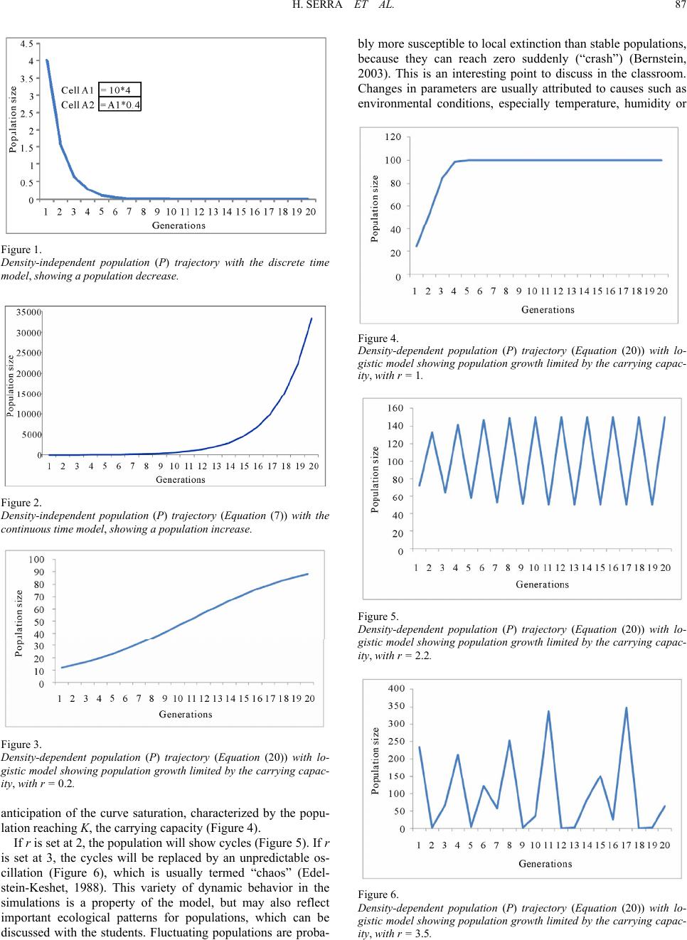

H. SERRA ET AL. 87
Figure 1.
Density-independent population (P) trajectory with the discrete time
model, showing a population decrease.
Figure 2.
Density-independent population (P) trajectory (Equation (7)) with the
continuous time model, showing a population increase.
Figure 3.
Density-dependent population (P) trajectory (Equation (20)) with lo-
gistic model showing population growth limited by the carrying capac-
ity, with r = 0.2.
anticipation of the curve saturation, characterized by the popu-
lation reaching K, the carrying capacity (Figure 4).
If r is set at 2, the population will show cycles (Figure 5). If r
is set at 3, the cycles will be replaced by an unpredictable os-
cillation (Figure 6), which is usually termed “chaos” (Edel-
stein-Keshet, 1988). This variety of dynamic behavior in the
simulations is a property of the model, but may also reflect
important ecological patterns for populations, which can be
discussed with the students. Fluctuating populations are proba-
bly more susceptible to local extinction than stable populations,
because they can reach zero suddenly (“crash”) (Bernstein,
2003). This is an interesting point to discuss in the classroom.
Changes in parameters are usually attributed to causes such as
environmental conditions, especially temperature, humidity or
Figure 4.
Density-dependent population (P) trajectory (Equation (20)) with lo-
gistic model showing population growth limited by the carrying capac-
ity, with r = 1.
Figure 5.
Density-dependent population (P) trajectory (Equation (20)) with lo-
gistic model showing population growth limited by the carrying capac-
ity, with r = 2.2.
Figure 6.
Density-dependent population (P) trajectory (Equation (20)) with lo-
gistic model showing population growth limited by the carrying capac-
ity, with r = 3.5.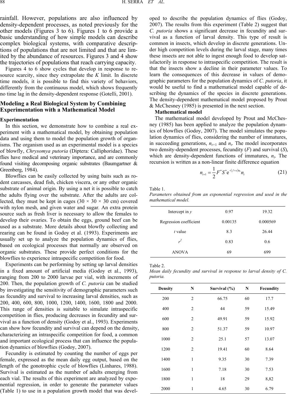

H. SERRA ET AL. 88
rainfall. However, populations are also influenced by
density-dependent processes, as noted previously for the
other models (Figures 3 to 6). Figures 1 to 6 provide a
basic understanding of how simple models can describe
complex biological systems, with comparative descrip-
tions of populations that are not limited and that are lim-
ited by the abundance of resources. Figures 3 and 4 show
the trajectories of populations that reach carrying capacity.
Figures 4 to 6 show cycles that develop in response to re-
source scarcity, since they extrapolate the K limit. In discrete
time models, it is possible to find this variety of behaviors,
differently from the continuous model, which shows frequently
no time lag in the density-dependent response (Gotelli, 2001).
Modeling a Real Biol o gi cal System by Combining
Experimentation with a Mathematical Model
Experimentation
In this section, we demonstrate how to combine a real ex-
periment with a mathematical model, by obtaining population
data and using them to model the population growth of organ-
isms. The organism used as an experimental model is a species
of blowfly, Chrysomya putoria (Diptera: Calliphoridae). These
flies have medical and veterinary importance, and are commonly
found visiting decomposing organic substrates (Baumgartner &
Greenberg, 1984).
Blowflies can be easily collected by using baits such as ro-
dent carcasses, dead fish, chicken viscera, or any other organic
substrate of animal origin. By using a net it is possible to catch
the adults flying over the substrate. After the adults are col-
lected, they must be kept in cages (30 × 30 × 30 cm) covered
with nylon mesh, and given water and sugar. An extra protein
source such as fresh liver is necessary to allow the females to
develop their ovaries. To obtain the eggs, ground beef can be
used as a substrate. More details about blowfly collecting and
rearing can be found in Godoy et al. (1993). Experiments are
usually set up to analyze the population dynamics of flies,
based on ecological processes that normally are observed on
organic substrates. These provide perfect conditions for the
blowflies to experience intraspecific competition for food.
Experiments can be performing by setting up larval densities
in a fixed amount of artificial media (Godoy et al., 1993),
ranging from 200 to 2000 larvae per vial, with increments of
200. Then, the population growth of C. putoria can be studied
by investigating the sensitivity of demographic parameters such
as fecundity and survival to increasing larval densities, such as
200, 400, 600, 800, 1000, 1200, 1400, 1600, 1800 and 2000.
This range of densities is suitable to simulate intraspecific
competition in flies, producing decreases in fecundity and sur-
vival as a function of density (Godoy et al., 1993). Experiments
can show how fecundity and survival can depend on the density,
characterizing an intraspecific competition for food, a common
and important ecological process that can influence the popula-
tion dynamics of blowflies (Godoy, 2007).
Fecundity is estimated by counting the number of eggs per
female, expressed as the mean daily egg output, based on the
length of the gonotrophic cycle of blowflies (Linhares, 1988).
Survival is estimated as the number of adults emerging from
each vial. The results of this experiment are analyzed by expo-
nential regression, in order to generate the parameter values
(Table 1) to use in a population growth model that was devel-
oped to describe the population dynamics of flies (Godoy,
2007). The results from this experiment (Table 2) suggest that
C. putoria shows a significant decrease in fecundity and sur-
vival as a function of larval density. This type of result is
common in insects, which develop in discrete generations. Un-
der high competition levels during the larval stage, many times
these insects are not able to ingest enough food to develop sat-
isfactorily in response to intraspecific competition. The result is
that the insects show a decline in their parameter values. To
learn the consequences of this decrease in values of demo-
graphic parameters for the population dynamics of C. putoria, it
would be useful to find a mathematical model capable of de-
scribing the dynamics of the species in discrete generations.
The density-dependent mathematical model proposed by Prout
& McChesney (1985) is presented in the next section.
Mathematica l mo del
The mathematical model developed by Prout and McChes-
ney (1985) has been applied to analyze the population dynam-
ics of blowflies (Godoy, 2007). The model simulates the popu-
lation dynamics of flies, considering the number of immatures,
in succeeding generations, nt+1 and nt. The model incorporates
two density-dependent processes, fecundity (F) and survival (S),
which are density-dependent functions of immatures, nt. The
recursion is written as a non-linear finite difference equation

1
1e
2
t
fsn
t
nFS


t
n (21)
Table 1.
Parameters obtained from an exponential regression and used in the
mathematical model.
Intercept in y 0.97 19.32
Regression coefficient 0.00135 0.000569
t value 8.3 26.44
r2 0.83 0.6
ANOVA 69 699
Table 2.
Mean daily fecundity and survival in response to larval density of C.
putoria.
Density N Survival (%) N Fecundity
200 2 66.75 60 17.7
400 2 44 59 15.49
600 2 49.91 59 15.92
800 2 51.37 59 10.97
1000 2 25.1 57 13.07
1200 2 19.41 60 8.64
1400 1 9.35 30 7.39
1600 1 7.18 30 7.53
1800 1 18 29 8,82
2000 1 4.65 30 6.79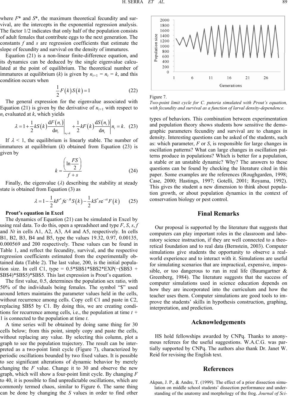

H. SERRA ET AL. 89
where F* and S*, the maximum theoretical fecundity and sur-
vival, are the intercepts in the exponential regression analysis.
The factor 1/2 indicates that only half of the population consists
of adult females that contribute eggs to the next generation. The
constants f and s are regression coefficients that estimate the
slope of fecundity and survival on the density of immatures.
Equation (21) is a non-linear finite-difference equation, and
its dynamics can be deduced by the single eigenvalue calcu-
lated at the point of equilibrium. The theoretical number of
immatures at equilibrium (k) is given by nt+1 = nt = k, and this
condition occurs when

11
2FkSk (22)
The general expression for the eigenvalue associated with
Equation (21) is given by the derivative of nt+1 with respect to
nt evaluated at k, which yields
 

 

dd
11
1
2d 2d
t
t
t
tt
nk
Fn Sn
kS kkF knk
nn


 .
t
(23)
If  < 1, the equilibrium is linearly stable. The number of
immatures at equilibrium (k) obtained from Equation (23) is
given by
ln 2
FS
k
f
s





(24)
Finally, the eigenvalue (  ) describing the stability at steady
state is obtained from Equation (3) as
 
**
11
1e e
22
fk sk
kFfSkkS sFk 

 (25)
Prout’s equation in Excel
The dynamics of Equation (21) can be simulated in Excel by
using real data. To do this, open a spreadsheet and type F, S, s, f
and Nt in cells A1, A2, A3, A4 and A5, respectively. In cells
B1, B2, B3, B4 and B5, type the values 19.32, 0.97, 0.00135,
0.000569 and 200 respectively. These values can be found in
Table 1, and reflect the fecundity, survival, and the respective
regression coefficients estimated from the experimentally ob-
tained data (Table 2). The last value, 200, is the initial popula-
tion size. In cell C1, type = 0.5*$B$1*$B$2*EXP(−($B$3 +
$B$4)*$B$5)*$B$5. This last expression is Prout’s equation.
The first value, 0.5, determines the population sex ratio, with
50% of the individuals being females. The symbol “$” used
around letters maintains the parameter values held in the cells,
without recurrence among cells. Copy cell C1 and paste in C2,
replacing $B$5 by C1. By doing this, we are creating condi-
tions for recurrence among cells, i.e., the population at time t +
1 is connected to the population at time t.
A time series will be obtained by doing same thing for 30
cells below; from this point, simply copy and paste the cells,
without replacing any value. By selecting this column, plot a
graph to see the population trajectory. The result can be inter-
preted as a two-point limit cycle (Figure 7), characterized by
periodic oscillations bounded by two fixed values. It is possible
to see significant alterations of dynamic behavior by merely
changing the F value. Change it to 30 and observe the new
graph, which will show a four-point limit cycle. By changing F
to 40, it is possible to find unpredictable oscillations, which are
commonly termed chaos, similar to Figure 6. The same thing
can be done by changing the S values in order to find other
Figure 7.
Two-point limit cycle for C. putoria simulated with Prout’s equation,
with fecundity and survival as a function of larval density-dependence.
types of behaviors. This combination between experimentation
and population theory shows students how sensitive the demo-
graphic parameters fecundity and survival are to changes in
density. Interesting questions can be asked of the students, such
as: which parameter, F or S, is responsible for large changes in
oscillation patterns? What can large changes in oscillation pat-
terns produce in populations? Which is better for a population,
a stable or an unstable dynamic? Why? The answers to these
questions can be found by checking the literature cited in this
paper. Some examples are the references (Roughgarden, 1998;
Case, 2000; Hastings, 1997; Gotelli, 2001; Royama, 1992).
This gives the student a new dimension to think about popula-
tion growth, or about population dynamics in the context of
conservation biology or pest control.
Final Remarks
Our proposal is supported by the literature that suggests that
computers can play important roles in the classroom and labo-
ratory science instruction, if they are well connected to a theo-
retical foundation and to real data (Bernstein, 2003). Computer
simulations give students the opportunity to observe a real-
world experience and to interact with it. Simulations are useful
for simulating scenarios that are impractical, expensive, impos-
sible, or too dangerous to run in real life (Baumgartner &
Greenberg, 1984). The literature suggests that the success of
computer simulations used in science education depends on
how they are incorporated into the curriculum and how the
teacher uses them. Computer simulations are good tools to im-
prove the students’ skills in hypothesis construction, graphing,
interpretation, and prediction.
Acknowledgements
HS hold fellowships awarded by CNPq. Thanks to anony-
mous referees for the useful suggestions. W.A.C.G. was par-
tially supported by CNPq. The authors also thank Dr. Janet W.
Reid for revising the English text.
References
Akpan, J. P., & Andre, T. (1999). The effect of a prior dissection simu-
lation on middle school students’ dissection performance and under-
standing of the anatomy and morphology of the frog. Journal of Sci-

H. SERRA ET AL. 90
ence Education and Technology, 8, 107-121.
doi:10.1023/A:1018604932197
Alessi, S. M., & Trollip, S. R. (1991). Computer based instruction:
Methods and development. Upper Saddle River, NJ: Prentice Hall.
Amabis, J. M., & Martho, G. R. (2005). Biologia de populações:
Genética, evolução e ecologia. São Paulo: Moderna.
Baumgartner, D. L., & Greenberg, B. (1984). The genus Chrysomya
(diptera: Calliphoridae) in the new world. Journal of Medical Ento-
mology, 21, 105-113.
Bell, R. L., Smetana, L., & Binns, I. (2005) Simplifying inquiry in-
struction. The Science Teacher, 72, 30-33.
Bernstein, R. (2003). Population ecology: An introduction to computer
simulations. Canada: John Wiley & Sons Canada, Ltd.
Breithach, K., & Maltas, J. (2003). An integrated curriculum in ad-
vanced mathematics/pre-calculus and physics. ULR (last checked 20
December, 2010).
http://www.pls.uni. edu/couch/integrated philosophy.htm
Cantrell, R. S., & Cosner, C. (2003). Spatial ecology via reaction-
diffusion equations. Chichester: John Wiley and Sons.
Case, T. J. (2000). An illustrated guide of theoretical ecology. New
York: Oxford University Press.
Castanho, M. J. P., Magnago, K. F., Bassanezi, R. C., & Godoy, W. A.
C. (2006). Fuzzy subset approach in coupled population dynamics of
blowflies. Biological Research, 39, 341-352.
doi:10.4067/S0716-97602006000200016
Edelstein-Keshet, L. (1988). Mathematical models in biology. New
York, NY: Random House.
Eykhoff, P. (1974). System identification: Parameter and State Estima-
tion. London: John Wiley & Sons.
Godoy, W. A. C. (2007). Dynamics of blowfly populations. Functional
Ecosystems and Communities, 1, 129-139.
Godoy, W. A. C., Reis, S. F., Von Zuben, C. J., & Ribeiro, O. B. (1993).
Population dynamics of Chrysomya putoria (wied.) (dipt. calliphori-
dae). Journal of Applied Entomology, 116, 163-169.
doi:10.1111/j.1439-0418.1993.tb01184.x
Gotelli, N. J. (2001). A primer of ecology (3rd ed.). Sunderland, Mas-
sachusetts: Sinauer Associates, Inc.
Green, J. L., Hastings, A., Arzberger, P., Ayala, F. J., Cottingham, K.
L., Cuddington, K., Davis, F., Dunne, J. A., Fortin, M. J., Gerber, L.,
& Neubert, M. (2005). Complexity in ecology and conservation:
Mathematical, statistical, and computational challenges. BioScience,
55, 501-510.
doi:10.1641/0006-3568(2005)055[0501:CIEACM]2.0.CO;2
Hastings, A. (1997). Population biology. New York, NY: Springer-
Verlag.
Hengeveld, R. (1989). Dynamics of biological invasions. New York,
NY: Chapman & Hall.
Hilborn, R., & Mangel, M. (1997). The ecological detective: Mono-
graphs in population biology. Princeton, NJ: Princeton University
Press.
Javidi, G. (2004). A comparison of traditional physical laboratory and
computer simulated laboratory experiences in relation to engineering
undergraduate students conceptual understandings of a communica-
tion systems topic. Ph. D. Thesis, Florida: University of South Florida.
(last checked 20 December, 2010)
http://scholarcommons.usf.edu/etd/2936.
Lima, E. A. B. F., Ferreira, C. P., & Godoy, W. A. C. (2009). Ecologi-
cal modeling and pest population management: A possible and nec-
essary connection in a changing world. Neotropical Entomology, 38,
699-707.
doi:10.1590/S1519-566X2009000600001
Linhares, A. X. (1988). The gonotrophic cycle of chrysomya mega-
cephala (diptera, calliphoridae) in the laboratory. Revista Brasileira
de Entomologia, 32, 383-392.
Murray, J. D. (2002). Mathematical biology. Washington: Springer,
Seattle.
Norris, D. (1994). Shortlist: A connectionist model of continuous
speech recognition. Cognition, 52, 189-234.
doi:10.1016/0010-0277(94)90043-4
Prout, T., & McChesney, F. (1985). Competition among immatures
affects their adult fertility: Population dynamics. American Natural-
ist, 126, 521-558. doi:10.1086/284436
Roughgarden, J. (1998). Primer of ecological theory. Upper Saddle
River, New Jersey: Prentice Hall.
Royama, T. (1992). Analytical population dynamics. London: Chapman
& Hall.
Schowalter, T. (2006). Insect ecology. Orlando: Academic Press.
Thompson, A., Simonson M., & Hardgrave, C. (1996). Educational
technology: A review of the research (2nd ed.). Washington, DC:
Association for Educational Communications and Technology.
Varaki, B. S. (2006). Math modeling in educational research: An ap-
proach to methodological fallacies. Australian Journal of Teacher
Education, 31, 29-35.
Wu, J., & David, J. L. (2002). A spatially explicit hierarchical approach
to modeling complex ecological systems: Theory and applications.
Ecological Modeling, 153, 7-26.
doi:10.1016/S0304-3800(01)00499-9
.
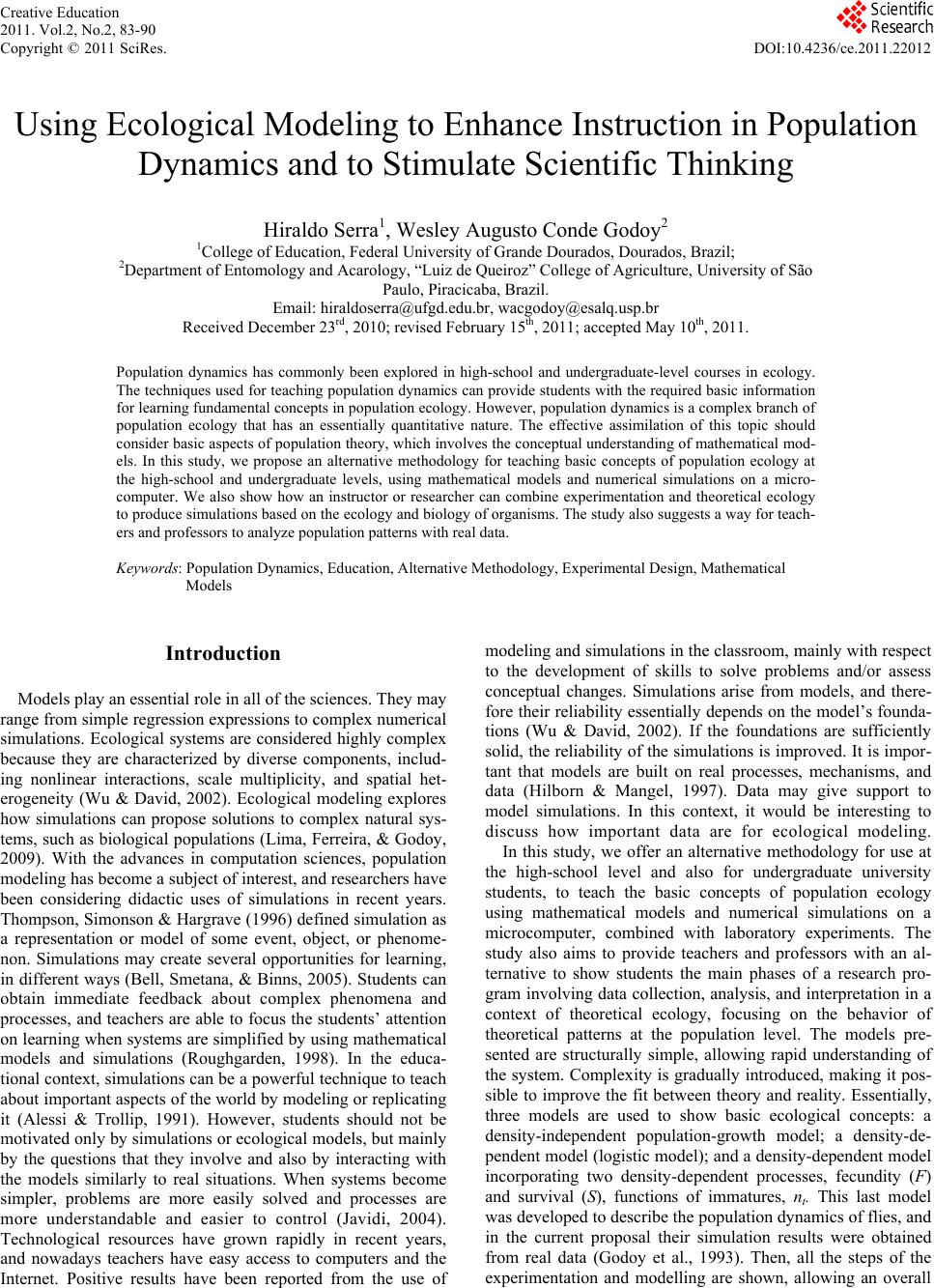