Received 19 November 2014

ABSTRACT

Studying the cosmic ray transport in the Galaxy, we deal with two interacting substances: charged particles and interstellar magnetic field. Two coupled local equations describe this complicated system, but elimination of one of them (say, the magnetic field equation) transforms remaining one (the cosmic rays equation) into the nonlocal form. The most popular nonlocal operators in the cosmic ray physics are integro-differential operators of fractional order. This report contains review of recent works in this direction, including original results of the author. In the last section, some specific problems are discussed: fractional operators with soft truncation of their kernels, nonlocal properties of fractional Laplacian, and a true form of the fractional material derivative.

Keywords:

Nonlocal Model, Anomalous Diffusion, Fractional Derivative, Fractal, Turbulence, Plasma, Cosmic Rays

1. Introduction

Cosmic rays were discovered in 1912 by Austrian scientist Victor Hess who made a series of ascents in a balloon to take measurements of radiation by using such simplest devices as electroscopes. Later, the use of more perfect apparatures allowed investigating cosmic rays at a wide variety of energies up to eV. The observed particle flux (number of particles per unit time per unit area) at Earth roughly follows a power energy spectrum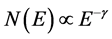,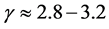. Detailed study of the energy spectra discovered some change in index at about eV (so-called the “knee”) which gave the basis for believing to cosmic rays originating from supernova explosions across the Galaxy. This large variation in observed particle energies implies that they originate from a variety of sources, but their weak anisotropy forces supposing its way being very intricate. Thus we observe a result of deep interplay existing between different cosmic components that continuously interact one another: the interstellar gas triggers star formation; massive stars generate Supernova explosions that accelerate cosmic rays; the gas returns back again in the interstellar medium and the released energy triggers the turbulence which is responsible for random walk of the cosmic ray. We will concentrate attention here only on the latter process.

For more complete mathematical treatment, the cosmic ray transport should be considered as a high-energy part of the cosmic plasma inheriting its main characteristic feature: turbulence. The turbulent interstellar magne- tic field has a crucial effect upon the CR transport, but the inverse influence is a bit weaker. Nevertheless, we deal with two interacting substances: charged particles (electrons, protons, nuclei) and magnetic field. Two coupled local equations describe this complicated system, but elimination of one of them (for instance, the magnetic field equation) transforms remaining one (in this case the cosmic rays equation) into an equation nonlocal with respect to spatial and time variables. The mathematical basement of this phenomenon is uncovered by the statistical mechanics. Let us cast an eye on its conclusion.

According to classical version of the Lindblad approach [1], a part of a closed Hamiltonian system is an open system governed by integrodifferential equation

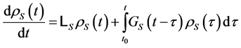
where is the phase density operator for and is the respective memory kernel. In case of long- range forces or free paths of particles, the time-nonlocality is naturally accompanied by the space-nonlocality. This way of thinking helps us to understand why transport of cosmic rays being a subsystem of the total electro- magnetic cosmic system (cosmic-ray particles + turbulent magnetic fields) is expected to be expressed in terms of nonlocal operators.

However, the Lindblad equation is rather abstract and doesn’t supply us by handy representation for the function. For this reason, I refer to the equation rather as a general idea than a real way for deriving the cosmic ray transport equation. Practically, until we get more information on interstellar media, the most reasonable way to state the problem ran through improvement of phenomenological models. In connection with this problem, it is very instructive to recall a Heisenberg article [2]. One of outstanding physicists-theorists of XX century defined a phenomenological theory as such a formulation of laws observed in physical phenomena, which does not attempt to completely reduce them to general fundamental “first principles”, through which they could be understood. The phenomenological theories played always a value-significant role in the development of physics. Referring to semi-empirical laws in meteorology, valency rules, interrelations between radii of atoms and ions, binding energies and excitation energies in chemistry, main interrelations in turbulent hydrodynamics, the Drude dispersive theory, phenomenological thermodynamics and Ptolemaic system in antique astronomy, Heisenberg wrote: “For technical and other applications, they were often more important than the apprehension of relations, and from a purely pragmatic point of view phenomenological theories can make the knowledge of nature laws to a large extent even redundant¹”. The closest to our topic phenomenological construction of such kind is the turbulence modeling. For this reason, I’ll consider primarily some cases of such kind in hydrodynamics and plasma physics.

2. Hydrodynamics

The simplest version of statistical description of molecular motion is based on equation

(1)

for propagator interpreted as a probability density function for a particle performing the Brownian motion. This is a random walk process with independent normally distributed increments, its variance is proportional to time.

Attempts to apply the model to the turbulent diffusion (say, in the see, or in the atmosphere) meet a few objections.

1. Trajectories of Brownian particles are continuous but nowhere differentiable so their intantaneous velo- cities are infinite.

2. This equation fails to describe the fact that a diffusion packet created by a local instantaneous source is bounded by the sphere linearly expanding with time.

3. The ordinary diffusion model gives a unique value for the eddy diffusivity, although it has been noted repeatedly that the phenomenological diffusivity is larger in proportion to the geometric scale of the experiment.

4. Unlike the molecular diffusion successfully described by Equation (1), turbulent flows and eddies introduce long-range spatial correlations in turbulent diffusion.

The first disadvantage is easily overcome by passing from the Brownian process to the Boltzmann process with piecewise constant velocity ν and exponentially distributed times of free motion. With this passage, the Fick current-concentration formula is replaced by the Maxwell-Cattaneo -interrelation:

where. But the exponential time-correlations look too short for the turbulent diffusion, and

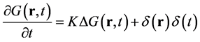
Bourret replaced by function of a more general type [3]. As a result, the propagator equation has taken the form

.

In case of anisotropic diffusion, scalar function is replaced by its tensor counterpart. determining mean-square displacement via relation

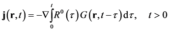
Concluding his article, Bourret wrote: “The absence of any spatial correlation term in our equation is conspicuous; consequently, use of the new formulation is probably justified only in application to regimes in which the spatial coherence is negligible in comparison with time coherence.” He amended the normal diffusion equation, replacing the classical Fick law by its nonlocal counterpart

With this generalization Bourett arrived at the integro-differential equation

(2)

Thus, in case of molecular diffusion in a dilute gas, a tracer interacts with almost independent molecules per collisions and this fact makes the diffusion equation local, but in the case of turbulent diffusion the motion of neighboring fluid elements is correlated, and the tracer motion continuously affected by the elements is described by the nonlocal Equation (2). The Fourier image of the correspondent Green equation reads

,.

Relying on turbulence scaling laws and dimensional analysis, Monin represented this equation in the following explicit form [4]

.

Later, the original of has been interpreted as an operator proportional to fractional Laplacian [5].

3. Plasma Physics

The following reasons provoke applying nonlocal models to problem of trasport in plasmas:

Ÿ Plasmas turbulence

Ÿ Trapping phenomena

Ÿ Fast propagation transport phenomena

Ÿ Scaling properties

Ÿ Non-Gaussianity and long-range correlations of fluctuations

Ÿ Anomalous diffusion and non-Gaussian pdfs in tracer transport studies.

There are published a few tens of works involving fractional derivatives as explicit form of nonlocal operators.

We shall touch on here some examples of them being more close to our metodology. Begin with the concept of a hybrid kinetic equation developed by Balescu [6]. In frame of this concept, the particle density function obeying the Vlasov equation with a random velocity field,

(3)

It reflects the same physics as the Langevin equation, but allows direct access to the distribution function. The latter is decomposed into the average (over the ensemble of realizations ) and the fluctuation:

(4)

Combining Equations (3), (4) and using the property yield the following system of coupled equation for the mean density function and for the fluctuation:

with the source term

After eliminating from the system the fluctuating part with applying the method of characteristics, Balescu arrived at the following integro-differential equation for a homogeneous and stationary turbulence:

This equation is of non-Markovian type with a memory kernel including by the Lagrangian velocity cor- relation tensor and a free term containing information on the initial fluctuation. If the initial condition of the distribution function is deterministic, , then the free term vanishes,.

Concluding his article, Balescu mentioned that in case of the weak turbulence the process becomes Markovian. When analysing strong turbulence, one needs to account the memory-function shape. It is conve- nient to be done if passing to propagator in its Laplace image:

(a particle is supposed to take the origin at the initial instant). Choosing (in frame of self-similar hypothesis) the kernel transformant in the power function form

multiplying both parts of the equation by and performing inverse Laplace transform, we arrive at a subdiffusion equation with partial time-derivative of fractional order

Thus, memory influence slows down a diffusion process meanwhile the Monin ansatz enhances it.

Combining both approaches leads to bifractional equation of anomalous diffusion

(5)

whose solutions are expressed via fractional stable distributions and cover both subdiffusive and superdiffusive regimes [7]. Detailed description of these distributions can be found in [8]. A series of works with application of Equation (5) to anomalous transport in turbulent plasmas are published by Sanches, Carreras, del Castillo-Negrete et al. (see review [9] and Reference therein).

Modeling of anomalous transport, typically based on gyrokinetic theory, is an essential tool for better understanding and possibly improving the confinement of magnetic fusion plasmas. An appropriate theoretical framework for high-temperature, low-density and thus weakly collisional fusion plasmas is provided by the gyrokinetic approach [10] where fast dynamics (e.g., the particle gyromotion) are eliminated from the full kinetic description but low-frequency physics is kept. In general, the resulting gyrokinetic Vlasov-Maxwell system of equations in low-dimensional phase space can only be solved numerically. Existing implementations can be classified into so-called local and global codes.

4. Isotropic Cosmic Ray Diffusion

4.1. Physical Causes of Nonlocality

In his first paper on the nature of cosmic rays, Fermi proposed a hypothesis that “cosmic rays are formed and accelerated mainly in the interstellar space, magnetic fields preventing them from coining out outside the Galaxy… Such fields are remarkably stable due to their large size (about a few light years) and comparatively high electric conductivity of the interstellar space. Indeed, the conductivity is so high that magnetic lines of force can be assumed “attached” to matter and involved in “flows” existing in it… There is evidence that this matter is distributed nonuniformly, the concentration of matter in some regions about 10 parsecs in size being 10 - 100 times higher… “Such relatively dense clouds occupy about 5% of the interstellar space” [11]. Fermi proved the acceleration mechanisms proposed by him in considering the motion of a particle in the interstellar space as a sequence of its scatterings in collisions with magnetized clouds.

Five years later, Ginzburg wrote: “The motion of charged particles in the interstellar space resembles Brownian motion or motion of molecules in a gas”. Indeed, due to the presence of the iterstellar magnetic field, in the region where this field is quasi-homogeneous, the trajectory of a particle winds around a magnetic field line and, upon averaging over the rotation period, is close to a straight line. However, on passing to a region with a different field direction, the trajectory changes and becomes a broken line as a whole. If the size of regions where the field direction noticeably changes is small compared to that of regions with a quasi-homogeneous field, the particle motion can be treated as the motion of a molecule in a gas: the motion is free in the homogeneous field, and a change in the velocity direction at a boundary is similar to a collision with another molecule and can be usually assumed instantaneous. Hence, the size of the region with a quasi-homogeneous field plays the role of the mean free path. The mean free time is, where is the translational velocity along the trajectory, which is by an order of magnitude equal to the usual velocity of the particle itself (and we therefore assume below that, where v is the particle velocity). If magnetic fields do not change in time, this collision process leads only to the diffusion of particles and the “mixing” of their velocities over directions but not to a change in the energy of the particles. It is known from the diffusion theory that the mean square distance passed by a particle in time is

where is the diffusion coefficient. According to astronomical data, cm in the interstellar medium, and for and (the proton lifetime), we obtain, which is of the

order of the size of the Galaxy. Therefore, for, protons, and all the more so nuclei, have no time to escape in great numbers from the Galaxy ([12], pp. 368, 369).

Beyond doubt, it was clear initially that the intricate cosmic-ray transfer process cannot be at all scales modeled by 3-dimensional Brownian motion. Assumption about increment independence of walking particle coordinates (in other words, of losing its memory) come into conflict with existing of more or less regular components of interstellar and interplanetary magnetic fields. In multiple scattering representation, forming the basis of the diffusion approximation, the particle free path distributions are not necessary to be exponential anymore but rather of inverse power kind as more typical for turbulent interstellar structures, This is directly linked with nonlocal operators in the form of fractional derivatives involving which for both space- and time-variables leads to bifractional Equation (6).

4.2. A Prelimit Form of the Bifractional Diffusion Equation

Let us come back to bifractional generalization of the normal diffusion Equation (5). Apart from space-time

variables, propagator depends on four parameters: orders of derivatives and length and time scale factors (and). The pair of latters define the “fractional diffusion coefficient”.

To understand the physical content of the equation, one can us turn to its Fourier-Laplace image:

Multiplyer can be counsidered as asymptotical expression for, where

(6)

Introducing and passing to prelimit form, we obtain algebraic equation

which in natural space-time variables takes the integral form:

(7)

As follows from Tauberian theorems, expressions (6) correspond toasymptotics

(8)

The physical sense of the prelimit equation becomes clear if we represent its solution as the Neumann series,

We see from here that the probability to find the particle at point of birth at time is equal to probability for the initial particle to stand motionless at this point until plus probability that it will make an instantaneous jump from the birth point to the point of observation at one of intermediate instants of time and will remain there until the time of observation, plus the probability to find at this point the particle after two instantaneous jumps separated by a random time interval with density, etc. If the distribution of coordinate jumps is of a power type with, the jumps are visible on all scales. A particle executing such a motion, “hangs around” for some time in the vicinity of relatively small sizes; then, it suddenly “flies away” to a large distance and “hangs around” a new vicinity. Motion of such kind is called “Lévy flights” (or Lévy motion, by analogy with Brownian motion), it named after the French mathematician who discovered the stable distributions.

4.3. Orders of Space-Time Fractional Operators

Among all characteristics of cosmic rays physics, only the energy spectra data cover more than ten orders of magnitude, whereas the ranges of other parameters are considerably smaller. A few irregularities observed in these spectra draw astrophysicists attention. In 2000, we found out that one of them―a change of the spectral index of the power law at an energy of about 4 PeV, the so called knee―appears when we pass from Gaussian statistics to Levy statistics and disappears when we return to the classical Gaussian. The Levy distribution densities result from equation with fractional Laplacian [7], which relates in common opinion to self-similar (fractal) inhomogeities of turbulent interstellar medium. We performed first numerical calculations in frame of this model

in 2000 [13]. With widely accepted assumption on the energy-dependence of diffusion coefficient and source energy spectrum, the spectrum at the distance from the point source aes com-

puted [14]. Analysis of these results has confirmed that something like knee is observed only in anomalous case, , and disappeared in frame of the normal diffusion model. In works [14] [15], we involved time-differential operator of fractional order with following comments: “Such choice of the distribution is motivated in the work [16] devoted to diffusion of solar magnetic elements. Its authors shown that is of inverse power type with. Distribution of such kind appear in some disordered solids and in percolation problems” ([14], p. 213). In the cosmic ray transport, time-fractional operator can be interpreted as an effect of magnetic traps confined charged particles. To determine the next important parameter, the anomalous diffusion coefficient, we used experimental data on the anisotropy of particle fluxes within the framework of the scheme proposed by Osborne et al. [17] and Dorman et al. [18]. In particular, we found that pc^1.7 year⁻⁰⁸ for and for the three nearest sources. In the model considered here, only one parameter , related to the fractal structure of the medium, was found by fitting. Test calculations of cosmic-ray spectra showed that the best fit of experimental data was achieved for.

Later, some authors used other values of the parameters but came back to these ones.

4.4. Walks with a Finite Velocity of Free Motion

Looking at Equation (7), we clearly see that the length of the jump vector and the time interval a particle stays in a trap are mutually independent: their joint distribution density is given by the product of their marginal densities:

Since the particle velocity is finite, the time spent on the jump itself should also be taken into account. Equation (7) will then take the form

(8)

If the times a particle stays in traps have a narrower power-law or exponential distribution than the mean free paths, then the latter will play a major role in the asymptotics of long times and the traps can be ignored, i.e., the particle can be assumed to move continuously with a velocity v constant in magnitude and changing in direction at ends of the mean free paths,

The corresponding propagator satisfies the equation

It was shown in [19] that the asymptotics of the solution of Equation (8) for and exponential trapping time distribution is expressed in terms of 3-dimensional stable distributions Lévy-Feldheim

(9)

with a simple substitution of the “diffusion coefficient”:

(10)

where, as above, denotes the velocity of free motion of the particle and is the mean path traversed by this particle per unit time provided that the jumps are instantaneous.

As regards the range, the situation is different. The mean free path is infinite, while its distribution is a power law. In the absence of a ballistic constraint (i.e., at), the diffusion packet represented by the self-similar solution of the fractional differential equation would spread proportionally to and would quickly go outside the ballistic boundaries for. The limited particle velocity prevents this; the ballistic boundaries squeeze the diffusion packet into a cone, imparting a characteristic W- or even S-shape to it [20]-[22].

The role of the ballistic constraints at clearly manifests itself in the asymptotic behavior of the

diffusion packet width. Assuming that the densities of the mean free path and the waiting time are characterized by asymptotics (9) and (10), we found in [23] [24] that

as.

4.5. Propagator with Ballistic Restriction

Whan random trajectories related to contains anomalously long rectilinear parts comparable with size of the Galaxy disc itself [25]-[27], and assumption on instantaneous flights to such distances looks to say the least of it unphysical. The exit from this situation lies in using the fractional material derivative operator as it described in the above-sited our works: this operator takes into account that cosmic ray particles propagate through interstellar medium with a finite speed. the fractional material operator used in our bounded anomalous diffusion model [28], where the following equations

;

for cosmic ray propagation were d. Here, the angle brackets denote averaging over all directions, and expression represents generalization of the material derivative. When, the equation

reduces in the long time asymptotic region to the Lévy-flight diffusion Equation (5) with and diffusivity (10) (see (9)).

5. Anisotropic Diffusion

5.1. Physical Causes of Nonlocality

Along with the isotropic model, the anisotropic diffusion model is used in local problems of galactic cosmic-ray transfer. This model was initially developed in theoretical studies of the motion of charged particles in quasihomogeneous regions with a fluctuating magnetic field slightly different from a constant homogeneous field. The development of this model led to the separation of the diffusion of charged particles into the longitudinal and transverse components, each of which was described by a diffusion equation of the corresponding dimension with its own diffusion coefficient. The transverse diffusion was the first example of anomalous diffusion. The transverse diffusion anomaly was manifested not only in its slowness compared to the normal diffusion (which could be achieved by simply introducing a smaller diffusion coefficient) but also in a different expansion law for a diffusion packet and its different shape. Some authors believe that the local interpretation of such a composite model of anomalous diffusion (compound diffusion) can be extended to the entire galactic disc. For example, Hayakawa writes: “In this model, interstellar magnetic fields are assumed almost homogeneous along spiral sleeves. Particles are drifting along field lines and are reflected at mirror points.... Particles captured and kept on a field line continue to diffuse in accordance with the chaotic motion of the field line.... Because the magnetic field is homogeneous only at the distance of a few kiloparsecs, we can assume that particles have escaped from the Galaxy if they have propagated a path longer than the field homogeneity length” [29].

Such patterns of the process inspire the idea of separate consideration these two stochastic motions: the particle motion along the line and the line deflection with regard to the initial straight line. This model called the compound diffusion model was firstly suggested by Russian astrophysicist Getmantsev [30] in 1963 and later investigated in details in [31]-[33]. We will call the standard compound model the case when longitudinal and lateral processes are described in frame of standard diffusion theory. In this case, the typical path of the particle

along the line during time is, and the lateral displacement of the line at this point is,

where is the longitudinal diffusivity of the particle, while denotes the lateral diffusivity of the line. As a result, we arrive at the equality

5.2. Propagators

Let be a longitudinal propagator, that is the pdf of longitudinal coordinate counting along field line at the moment under the initial condition, and be a pdf of the lateral

displacement of magnetic line at the point (is a two-dimensional vector). The resulting lateral pdf is given by the Chapman-Kolmogorov equation:

In frame of standard compound model, the longitudinal propagator and pdf of lateral displacements of magnetic field line obey the ordinary one-dimensional and two-dimensional diffusion equations respectively:

Zaburdaev [34] has shown that the random-walk process just considered, namely, the one whose argument is also a random-walk process, obeys a subdiffusion scaling, as follows. Considering an initial particle distribution as uniform along the -axis and keeping in mind, that in this situation, particles with different coordinates can occur at the same magnetic field line, he writes down the total concentration as

Taking the Fourier-Laplace transform with respect to space-time variables yields

In terms of space-time variables, this expression relates to the fractional differential equation

The author concludes his article by noting that “the problem considered above constitutes one of the few examples of the rigorous derivation of an equation with fractional derivatives and thereby shows the naturalness and importance of this approach to describing stochastic processes in which the subdiffusive behavior of the particles is an inherent feature of the physical phenomenon” [34].

It is necessary to say that in general the actions of random walk of the magnetic field lines and random particles motions are not independent. So, strictly speaking, these processes should be studied together. Such consideration first carried out by Chuvilgin and Ptuskin [32] has led to the fractional subdiffusion equation.

5.3. Longitudinal Propagator with Ballistic Restriction

Reconsider the random walk of particles along magnetic field linestaking into account that the particle moves with a finite velocity. Assuming that the time needed for particles to pass between lines is small, the longitudinal motion can be considered as a continuous one although may reverse the direction at random instants of time. The one-dimensional symmetric random walk of a particle with a constant velocity along -axis in the absence of traps is completely characterized by the distribution density of its free paths. In a medium consisting of uniformly distributed independent scatterers, free paths are distributed according to the exponential law, and the process is governed by a second-order partial differential equation (the telegraph equation) [35]. The solution of this equation is expressed in terms of the modified Bessel functions and transforms into the normal (Gaussian) distribution in the asymptotic regime of large times. In Refs. [36]-[38], authors investigated one-

dimensional random walks with the asymptotically power-law distribution, , which are

sometimes called fractal walks. Here, we shortly itemize the different propagators which can be used for description of longitudinal walk of guiding center.

The simplest ballistic transport model describes free motion of particles along a magnetic field line so in a simmetric case we have

This anzatz gives

for the particle transport across the field, where the perpendicular diffusion coefficient. Thus, ballistic transport of particles along the field, coupled with normal diffusion of lines, gives normal perpendicular diffusion for the particles across the field, with diffusion coefficient. Taking normal diffusion model for paralled transport,

,

we arrive at the original Getmantzev compound model, leading to subdiffusion process of lateral broadening of the cosmic rays packet. However, this model is not in a position to describe the ballistic regime of motion doubtless existing at small scales.

In [38], we investigated asymmetrical one-dimensional random walks with finite constant speed and the

asymptotically power-law distribution of path length, and probabilities and for scattering to the right and to the left respectively. In case its asymptotics reads

Thus, the equation for longitudinal propagator is of the form

Its solution reads

In case first moment exists, and asymptotic expression for the propagator is represented by means of one-dimentional -stable density [39].

6. Some Problems and Perspectives

In conclusion, I’d like to make a short comment to foundation of the nonlocal approach and to list some problems connected with further development of the method.

Recall that the habitual distributon, originates from the model of an ideal gas molecules of which are placed independently of each other. However, this representation does not always work. For example, it is inapplicable for transport of particles in directions close to axis in crystal structures, because positions of atoms in such structures are not independent of each other. The same takes place and in transport of particles along field lines: turning points are situated close to these lines and there is not any evidence that random distances between them are distributed according to exponential law, whereas, the power-type distribution looks more naturally in the company of other power-type laws related to turbulent media.

The following problems seem to be very actual now to me.

1. First of them concerns the distribution of waiting time. Numerical simulation of the trajectories of particles in a turbulent plasma has shown [40] that charged particles are indeed captured by vortices (“traps”) formed in the turbulent plasma and are confined in them for a long time. This time is random, and its probability distribution is characterized by a sufficiently long power-law region, but this region is restricted from both sides. Introduction of correction in form of some truncations is more or less soft; we obtain an equation with first-order time derivative for long-time asymptotics. These two regions can be combined in a single equation in the case of soft decay by introducing an exponential factor in the kernel of the fractional differential operator [41]:

The subdiffusion equation becomes then

It is clear that this effect can be obtained not only for the exponential but also for other factors providing a rapid decay (or indeed termination) of the asymptotic part of the power-law distribution, such that the mean time would become finite; the exponential factor can easily be incorporated into the result due to the use of the Laplace transform.

2. A similar problem takes place with the fractional Laplacian, because the power-law spectrum on which its representation is based is valid only in a limited range of wave numbers, whereas the fractional Laplacian itself should possess the power-law spectrum at all scales. On assumption that the divergence of free paths moments begins with the next, the fourth order, the fractional generalization of the transport equation takes the form

(11)

The inclusion of the additional term in the equation violates the important property of the self-similarity of its solutions, but at the same time imparts an interesting feature to it. The process described by Equation (11) describes the ordinary diffusion at large scales but subdiffusion at small scales. The same equation with α from the lower range,

describes usual diffusion at smaller scales and superdiffusion at larger scales. The difference between these processes is explained, of course, by the different properties of the medium at different scales.

3. Unlike the usual Laplacian whose form is independent of boundaries and

boundary conditions, the fractional Laplacian depends on them. In the fractional Laplacian, it is necessary to specify not only the properties of the sought function at the domain boundaries, but also its values outside this

domain. The popular Fourier transform of the fractional Laplacian in a bounded medium is no longer

applicable. In this case, the interpretation in terms of flights is very useful for determining the influence of the boundary quality (reflecting, transparent, semitransparent, diffusive) on the solution and for better understanding characteristics that are not so obvious, such as the times the boundary first reaches and first passes through. We note that the expansion of the Laplacian in Cartesian or other orthogonal coordinates, providing a theoretical basis for the method of separation of variables, is not applicable in the fractional differential case: the fractional three-dimensional Laplacian cannot be written as a sum of one-dimensional Laplacians along, , and.

.

Similarly, it is impossible to separate the fractional Laplacian into the radial and angular components. The use of only a radial fractional Laplacian in any equation can only mean that the motion only along radial trajectories is considered, whereas in the case of the usual Laplacian, its radial component reflects the evolution of the radial coordinate of a complex spatial trajectory.

The authors of [42] introduced a matrix representation of the one-dimensional fractional Laplacian, which was used for numerical solutions of problems with absorbing boundaries. The fractional Laplacian in presence of a reflecting wall is found in [43]. In [44], the fractional Laplacian was introduced as the generalization of the one-dimensional expression for the fractional Marchaud derivative to a bounded domain of the -dimensional space. The authors of [45], who studied reflected symmetric stable processes, involved concept of the regional fractional Laplacian.

Because of the abovementioned difficulties encountered in the consideration of boundary conditions, the best method for formulating boundary value problems in the nonlocal theory is still based on the use of integral equations and Monte Carlo simulations.

4. As soon as we pass to the kinetic description (“include velocity”), the partial derivative transforms into the material derivative. In the fractional differential approach, this gives rise to the trans- formation. This fractional operator cannot be represented as a linear combination of partial fractional operators, , , , as some authors do. One should indicate a line,

along which we are going to compute this derivative (see for detail [46]).

I hope that successful solving of the listed problems will stimulate further development of the nonlocal transport theory reviewed in this article.

Acknowledgements

Author is grateful to the Russian Foundation for Basic Research (project no. 13-01-00585) and the Ministry of Education and Science of the Russian Federation (2014/296) for financial support.

Cite this paper

Vladimir V. Uchaikin, (2015) Nonlocal Models of Cosmic Ray Transport in the Galaxy. Journal of Applied Mathematics and Physics,03,187-200. doi: 10.4236/jamp.2015.32029

References

NOTES

¹Not wanting to give an absolute sense of the latter assertion, we would like to emphasize his trust relationship to phenomenological theories.

References

- 1. Lindblad, G. (1976) On the Generators of Quantum Dynamical Semigroups. Communications in Mathematical Physics, 48, 119-130. http://dx.doi.org/10.1007/BF01608499
- 2. Heisenberg, W. (1966) Die Rolle dor ph?nomenologischen Theorien im System der theoretischen Physik. In: Preludes in Theoretical Physics, Amsterdam, 166.�
- 3. Bourret, R. (1959) An Hypothesis Concerning Turbulent Diffusion. Canad. J. Phys, 38, 665-676. http://dx.doi.org/10.1139/p60-072
- 4. Monin, A.S. (1955) Equation of Turbulent Diffusion. Dokl. Akad. Nauk SSSR, 105, 256-259.
- 5. Monin, A.S. and Yaglom, A.M. (1975) Statistical Fluid Mechanics. Mechanics of Turbulence Vol. 2, MIT Press, Cambridge. [Translated from Russian: Statisticheskaya Gidromekhanika. Mekhanika Turbulentnosti Part 2 (Nauka, Moscow, 1967)]
- 6. Balescu, R. (2000) Memory Effects in Plasma Transport Theory. Plasma Phys. Control. Fusion, 42, B1-B13. http://dx.doi.org/10.1088/0741-3335/42/12B/301
- 7. Uchaikin, V.V. and Zolotarev, V.M. (1999) Chance and Stability. Stable Distributions and Their Applications. VSP, Utrecht. http://dx.doi.org/10.1515/9783110935974
- 8. Uchaikin, V.V. (2002) Multidimensional Symmetric Anomalous Diffusion. Chemical Physics, 284, 507-520. http://dx.doi.org/10.1016/S0301-0104(02)00676-6
- 9. del Castillo-Negrete, D. (2010) Non-Diffusive, Nonlocal Transport in Fluids and Plasmas. Nonlin. Processes Gheophys., 17, 795-807. http://dx.doi.org/10.5194/npg-17-795-2010
- 10. Brizard, A.J. and Hahm, T.S. (2007) Foundations of Nonlinear Gyro-kinetic Theory. Reviews of Modern Physics, 79, 421-469. http://dx.doi.org/10.1103/RevModPhys.79.421
- 11. Str?mgren, B. (1948) On the Density Distribution and Chemical Composition of the Interstellar Gas. Astrophys. J., 108, 242-275. http://dx.doi.org/10.1086/145068�
- 12. Ginzburg, V.L. (1953) Origin of Cosmic Rays and Radioastronomy. Usp.Fiz.Nauk, 51, 343. (In Russian)
- 13. Lagutin, A.A., Nikulin, Yu.A. and Uchaikin, V.V. (2001) The ?knee? in the Primary Cosmic Ray Spectrum as Consequence of the Anomalous Diffusion of the Particles in the Fractal Interstellar Medium. Nucl. Phys. В Proc. Suppl., 97, 267-270.�
- 14. Lagutin, A.A. and Uchaikin, V.V. (2003) Anomalous Diffusion Equation: Application to Cosmic Ray Transport. Nucl. Instrum. Meth. Phys. Res., 201B, 212-216. http://dx.doi.org/10.1016/S0168-583X(02)01362-9
- 15. Lagutin, A.A., Strelnikov, D.V. and Tyumentsev, A.G. (2001) Mass Composition of Cosmic Rays in Anomalous Diffusion Model: Comparison with Experiment. Proc. of 27th Intern. Cosmic Ray Conf., Hamburg, Germany, 5, Copernicus Gesellschaft, Ham-burg.
- 16. Cadavid, A.C., Lawrence, J.K. and Ruzmaikin, A.A. (1999) Anomalous Diffusion of Solar Magnetic Elements. Astrophys. J, 521, 844-853. http://dx.doi.org/10.1086/307573
- 17. Osborne, J.L., Wdowczyk, J. and Wolfendale, A.W. (1976) Origin and Propagation of Cosmic Rays in the Range 100 - 1000 GeV. J. Phys. A Math. Gen., 9, 1399-1412. http://dx.doi.org/10.1088/0305-4470/9/8/030
- 18. Dorman, L.I., Ghosh, A. and Ptuskin, V.S. (1985) Diffusion of Galactic Cosmic Rays in the Vicinity of the Solar System. Astrophys. Space Sci., 109, 87-98. http://dx.doi.org/10.1007/BF00651016
- 19. Zolotarev, V.M., Uchaikin, V.V. and Saenko, V.V. (1999) Superdiffusion and Stable Laws. JETP, 88, 780-787. http://dx.doi.org/10.1134/1.558856
- 20. Uchaikin, V.V. and Sibatov, R.T. (2004) Fractional Derivatives in the Semi-conductor Theory. Technical Physics Letters, 30, 316-318. http://dx.doi.org/10.1134/1.1748611
- 21. Uchaikin, V.V. and Sibatov, R.T. (2009) Statistical Model of Fluorescence Blinking. JETP, 109, 537-546. http://dx.doi.org/10.1134/S106377610910001X
- 22. Uchaikin, V.V., Sibatov, R.T. (2011) Fractional Boltzmann Equation for Multiple Scattering of Resonance Radiation in Low-Temperature Plasma. J. Phys. A Math. Theor., 44, 145501. http://dx.doi.org/10.1088/1751-8113/44/14/145501
- 23. Uchaikin, V.V. (1998) Anomalous Diffusion of Particles with a Finite Free-Motion Velocity. Theoretical and Mathematical Physics, 115, 496-501. http://dx.doi.org/10.1007/BF02575506
- 24. Uchaikin, V.V. (1998) Anomalous Transport Equations and Their Application to Fractal Walking. Physica A, 255, 65-92. http://dx.doi.org/10.1016/S0378-4371(98)00047-8
- 25. Uchaikin, V.V. and Sibatov, R.T. (2012) On Fractional Differential Models for Cosmic Ray Diffusion. Gravitation Cosmology, 18, 122-126. http://dx.doi.org/10.1134/S0202289312020132
- 26. Uchaikin, V.V., Sibatov, R.T. and Saenko, V.V. (2013) Escape Time of Cosmic Rays from the Galaxy in the Anomalous Diffusion Model. Bulletin of the Russian Academy of Sciences: Physics, 77, 619-622. http://dx.doi.org/10.3103/S1062873813050511
- 27. Uchaikin, V.V., Sibatov, R.T. and Saenko, V.V. (2013) Leaky-Box Approximation to the Fractional Diffusion Model. J. Phys.: Conf. Ser., 409, 012057.
- 28. Uchaikin, V.V. (2010) On the Fractional Derivative Model of the Transport of Cosmic Rays in the Galaxy. JETP Lett., 91, 105-109. http://dx.doi.org/10.1134/S002136401003001X
- 29. Hayakawa, S. (1969) Cosmic Ray Physics; Nuclear and Astro-physical Aspects. Wiley-Interscience, New York.
- 30. Getmantsev, G.G. (1963) On the Isotropy of Primary Cosmic Rays. Sov. Astron., 6, 477-479.
- 31. Jokipii, J.R. and Parker, E.N. (1969) Cosmic-Ray Life and the Stochastic Nature of the Galactic Magnetic Field. Astrophys. J., 155, 799.
- 32. Chuvilgin, L.G. and Ptuskin, V.S. (1993) Anomalous Diffusion of Cosmic Rays across the Magnetic Field. Astronomy and Astrophysics, 279, 278-297.
- 33. Webb, G.M., Kaghashvili, E.K., Le Roux, J.A., Shalchi, A., Zank, G.P. and Li, G. (2009) Compound and Perpendicular Diffusion of Cosmic Rays and Random Walk of the Field Lines: II. Non-Parallel Particle Transport and Drifts. Journal of Physics A: Mathematical and Theoretical, 42, 235502. http://dx.doi.org/10.1088/1751-8113/42/23/235502
- 34. Zaburdaev, V.Y. (2005) Theory of Heat Transport in a Magnetized High-Temperature Plasma. Plasma Physics Reports, 31, 1071-1077. http://dx.doi.org/10.1134/1.2147653
- 35. Uchaikin, V.V. and Saenko, V.V. (2000) Telegraph Equation in Random Walk Problem. Journal of Physical Studies, 4.
- 36. Shlesinger, M.F., Klafter, J. and West, B. (1986) Lévy Walks with Applications to Turbulence and Chaos. Physica A: Statistical Mechanics and its Applications, 140, 212-218.
- 37. Sokolov, I.M. andMetzler, R. (2003) Towards Deterministic Equations for Lévy Walks: The Fractional Material Derivative. Physical Review E, 67, 010101. http://dx.doi.org/10.1103/PhysRevE.67.010101
- 38. Uchaikin, V.V. and Sibatov, R.T. (2004) One-Dimensional Fractal Walk at a Finite Free Motion Velocity. Technical Physics Letters, 30, 316-318. http://dx.doi.org/10.1134/1.1748611
- 39. Uchaikin, V., Sibatov, R. and Byzykchi, A. (2014) Cosmic Rays Propagation along Solar Magnetic Field Lines: A Fractional Approach. Communications in Applied and Industrial Mathematics, 6, 480. http://dx.doi.org/10.1685/journal.caim.480
- 40. Carreras, В.A., Lynch, V.E. and Zaslavsky, G.M. (2001) Anomalous Diffusion and Exit Time Distribution of Particle Tracers in Plasma Turbulence Model. Phys. Plasmas, 8, 5096.
- 41. Sibatov, R.T. and Uchaikin, V.V. (2011) Truncated Lévy Statistics for Dispersive Transport in Disordered Semiconductors. Commun. Nonlin. Sci. Numer. Simulat, 16, 4564-4572. http://dx.doi.org/10.1016/j.cnsns.2011.03.027
- 42. Zoia, A., Rosso, A. and Kardar, M. (2007) Fractional Laplacian in Bounded Domains. Phys. Rev. E, 76, 021116. http://dx.doi.org/10.1103/PhysRevE.76.021116
- 43. Krepysheva, N., Di Pietro, L. and Neel, M.-C. (2006) Space-Fractional Advection-Diffusion and Reflective Boundary Condition. Phys. Rev. E, 73, 021104. http://dx.doi.org/10.1103/PhysRevE.73.021104
- 44. Rafeiro, H. and Samko, S. (2008) Approximative Method for the Inversion of the Riesz Potential Operator in Variable Lebesgue Spaces. Fract. Calc. Appl. Anal, 11, 269-280.
- 45. Guan, Q.-Y. and Ma, Z.-M. (2005) Boundary Problems for Fractional. Stoch. Dyn., 5, 385. http://dx.doi.org/10.1142/S021949370500150X
- 46. Uchaikin, V.V. (2013) Fractional Phenomenology of Cosmic Ray Anomalous Diffusion. Physics-Uspekhi, 56, 1074- 1119. http://dx.doi.org/10.3367/UFNe.0183.201311b.1175
NOTES
1Not wanting to give an absolute sense of the latter assertion, we would like to emphasize his trust relationship to phenomenological theories.