Vol.3, No.6, 419-425 (2011) Natural Science
http://dx.doi.org/10.4236/ns.2011.36057
CFD evaluation of thermal convection inside the DACON
convection sensor in actual space flight
Pradyumna Ghosh, Mihir Kumar Ghosh
Department of Mechanical Engineering Institute of Technology, Banaras Hindu University (BHU), Varanasi, India;
Received 2 February 2011; revised 15 March 2011; accepted 27 March 2011.
ABSTRACT
A CFD(Computational Fluid Dynamics) model
has been developed using the commercial CFD
package FLUENT for the thermal convection
inside air filled cylindrical DACON sensor,
where the onboard time dependent gravitational
micro acceleration has been considered. Time
dependent, curve fitted gravitational accelera-
tion in x- and y-axes from published data have
been incorporated in FLUENT through a User
Defined Function (UDF), developed in C which
includes space craft rotation. At the sensor
plane the two-dimensional flow has also been
visualized. A good agreement is between simu-
lation and published experimental data. Last but
not the least, for checking its response to suffi-
ciently strong perturbations in an orbital flight,
physical and numerical experiments are carried
out where an astronaut swung the sensor in
hands along the y axis with amplitude of 10cm
and a frequency of 0.2 Hz. A good qualitative
validation has been achieved between CFD and
actual experimental results.
Keywords: CFD (Computational Fluid Dynamics);
DACON sensor; Experimental Data; FLUENT; UDF
(User Defined Functions)
1. INTRODUCTION
Microgravity indicates low gravity, where the mean
gravitational acceleration is in the range of 10–1 - 10–5
m/s2. All on-board experiments in the automatic and
manned spacecraft experience residual micro-accelera-
tions or g-jitter. These micro-accelerations are most sig-
nificant in the frequency range 0 - 0.01 Hz. Internal nat-
ural convection is a phenomenon of natural convection
in an enclosure which has immense potential of engi-
neering application. In this connection, DACON con-
vection sensor has been developed to measure the re-
sponse of micro-acceleration in the buoyancy driven
thermal convection characteristics [1-5].
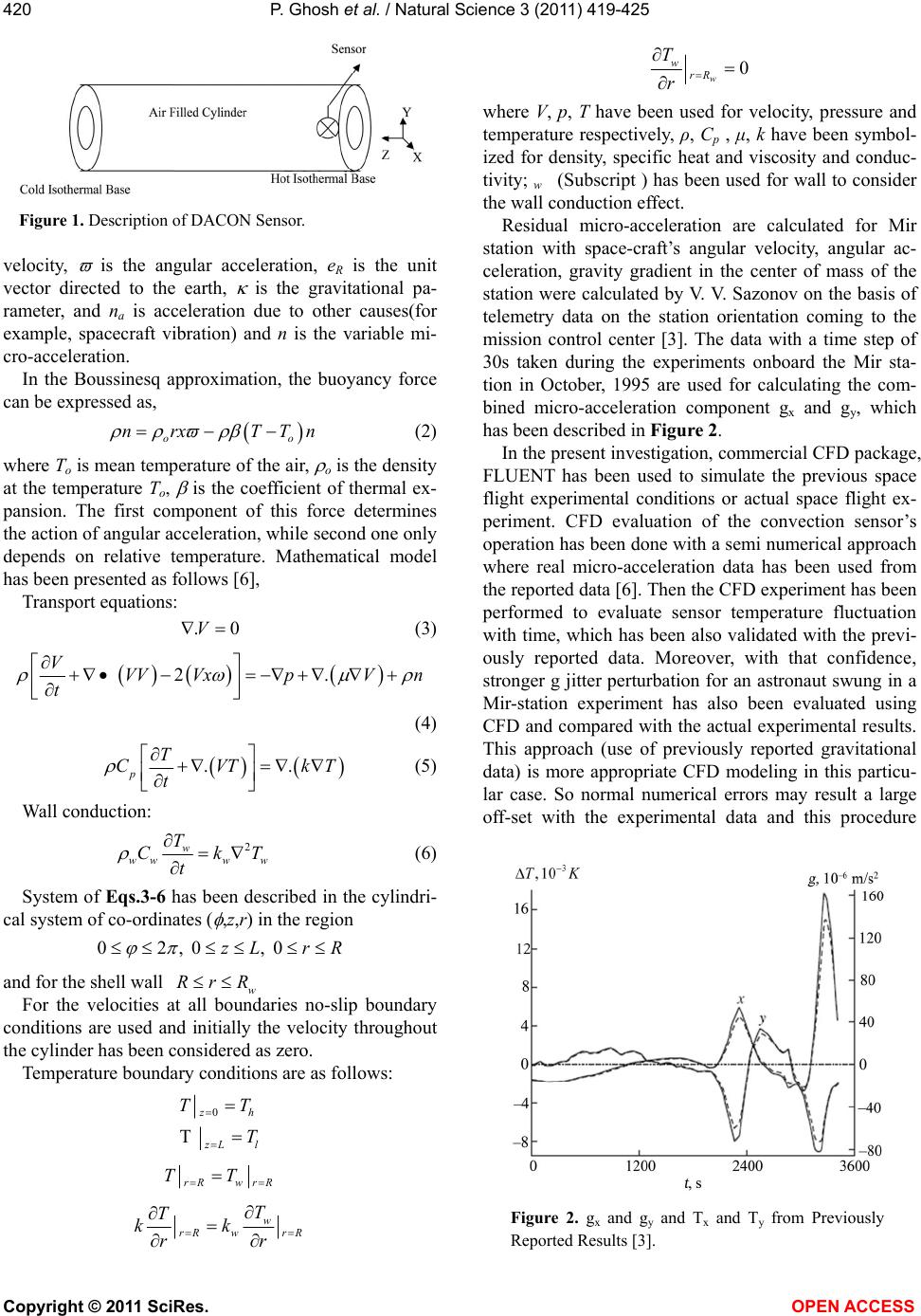
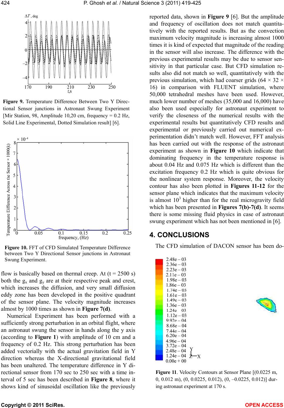
DACON convection sensor, shown in Figure 1, is an
air-filled cylindrical cavity of strictly controlled bound-
ary conditions for quick calculation of temperature field
under real space flight conditions (under on-board mi-
cro-acceleration). The wall thickness of the cylinder is
2.5 mm and the thermal conductivity of the wall material
is in the range of 0.16 - 2.3 W/m-K. The junctions of the
temperature sensors have been located 10 mm from the
hotter isothermal wall at a diameter of 45 mm, where the
entire cylindrical curved surface is adiabatic [6].
These two crossed differential temperature sensor
probes are placed in the cylindrical cavity in such a way
that their sensitivity axis are perpendicular to the cylin-
der axis, where as constant temperature difference was
maintained between the cylinder bases in actual space
flight situation. In satellites and orbital stations mi-
cro-gravity oscillation has been felt as a consequence of
spacecraft rotation, crew activity, different kind of vibra-
tion, non-uniformities of the earth’s gravitational field
etc. So far most of the studies have been concerned with
the convection under constant reduced gravity or har-
monic gravity vibration (g jitter). However the actual
behavior of fluid under orbital flight conditions is more
complicated. Indeed, the space craft rotation not only
contribute to the resultant vector micro-accelerations,
but also gives rise to additional forces which cannot be
reduced to some equivalent buoyancy forces.
In case of internal natural convection under sinusoidal
g-jitter streaming flow has been observed where pulsat-
ing wave from hot and cold side travels towards the cen-
tre and engages in constructive/destructive interface to
the formation of stationary wave [7].
The variable micro-acceleration due to rotation, angu-
lar acceleration and the gravity gradient can be ex-
pressed as [4-6],


3.
RR
nnaxrxw rxerer 

  

(1)
where r is the radius vector of a point,  is its angular

P. Ghosh et al. / Natural Science 3 (2011) 419-425 420
Figure 1. Description of DACON Sensor.
velocity,
 is the angular acceleration, eR is the unit
vector directed to the earth,
 is the gravitational pa-
rameter, and na is acceleration due to other causes(for
example, spacecraft vibration) and n is the variable mi-
cro-acceleration.
In the Boussinesq approximation, the buoyancy force
can be expressed as,


oo
nrx TTn   (2)
where To is mean temperature of the air, 
o is the density
at the temperature To,
 is the coefficient of thermal ex-
pansion. The first component of this force determines
the action of angular acceleration, while second one only
depends on relative temperature. Mathematical model
has been presented as follows [6],
Transport equations:
.0V (3)
 
2.
VVVVxpV n
t




 



(4)
 
..
p
T
CVTkT
t







(5)
Wall conduction:
2 w
wwww
T
CkT
t


 (6)
System of Eqs. 3-6 has been described in the cylindri-
cal system of co-ordinates (  ,z,r) in the region
02, 0, 0zL rR

  
and for the shell wall w RrR
For the velocities at all boundaries no-slip boundary
conditions are used and initially the velocity throughout
the cylinder has been considered as zero.
Temperature boundary conditions are as follows:
0
T
z
h
z
Ll
TT
T




rR wrR
TT


w
rR wrR
T
T
kk
rr




0
w
w
rR
T
r


where V, p, T have been used for velocity, pressure and
temperature respectively, ρ, Cp , μ, k have been symbol-
ized for density, specific heat and viscosity and conduc-
tivity; w (Subscript ) has been used for wall to consider
the wall conduction effect.
Residual micro-acceleration are calculated for Mir
station with space-craft’s angular velocity, angular ac-
celeration, gravity gradient in the center of mass of the
station were calculated by V. V. Sazonov on the basis of
telemetry data on the station orientation coming to the
mission control center [3]. The data with a time step of
30s taken during the experiments onboard the Mir sta-
tion in October, 1995 are used for calculating the com-
bined micro-acceleration component gx and gy, which
has been described in Figure 2.
In the present investigation, commercial CFD package,
FLUENT has been used to simulate the previous space
flight experimental conditions or actual space flight ex-
periment. CFD evaluation of the convection sensor’s
operation has been done with a semi numerical approach
where real micro-acceleration data has been used from
the reported data [6]. Then the CFD experiment has been
performed to evaluate sensor temperature fluctuation
with time, which has been also validated with the previ-
ously reported data. Moreover, with that confidence,
stronger g jitter perturbation for an astronaut swung in a
Mir-station experiment has also been evaluated using
CFD and compared with the actual experimental results.
This approach (use of previously reported gravitational
data) is more appropriate CFD modeling in this particu-
lar case. So normal numerical errors may result a large
off-set with the experimental data and this procedure
Figure 2. g
x and gy and Tx and Ty from Previously
Reported Results [3].

P. Ghosh et al. / Natural Science 3 (2011) 419-425 421
will reduce the probability of it, as one of the compo-
nents of numerical calculation is pre verified. Thus CFD
simulation provides more insight of the natural convec-
tion physics under actual g-jitter which had not been
even captured through the physical experiment.
2. CFD MODELING
Firstly, an effort has been made to study the convec-
tion in the cylinder with hotter and colder isothermal
bases with the entire adiabatic cylindrical curved surface,
temperature difference in the thermocouple junctions
under quasi-steady acceleration based on real micro-
gravity field data. The CFD experiment has been ex-
posed to real acceleration field. The cylindrical volume
with a wall thickness of 2.5 mm as shown in Figure 3
has been finely meshed with tetrahedral volume meshes
and four iso-point surfaces have been created in such a
way that their sensitivity axis are perpendicular to the
cylinder axis (z axis) to simulate the thermocouple junc-
tions in GAMBIT. It has been observed that, mesh fine-
ness increases the sensitivity of the sensor and as the
DACON sensor has a very low sensitivity finest possible
mesh has been used to capture the smaller fluctuation in
scalar variables and eventually that increases the com-
putation time.
These iso-point surfaces are located 10 mm away
from the hot isothermal base at a radius of 45 mm as
shown in Figure 4.
Like many other natural-convection flows, for faster
convergence Boussinesq model has been used. This
model treats density as a constant value (which has been
supplied as the Material Property taking air as a working
fluid) in all transport equations, except for the buoyancy
term in the momentum equation. As the Boussinesq ap-
proximation is only valid when the temperature differ-
ence between the hotter and cooler wall is less where as
for the present numerical experimentation that has been
always considered as 50˚C for air as working fluid [1,6].
All the relevant material properties for working fluid and
Figure 3. Meshed Cylindrical Air Filled
Volume with Sensor Point Surfaces.
Figure 4. Relative position of temperature
sensor with respect to hotter isothermal cy-
lindrical base.
Table 1. Thermophysical properties of the working fluid.
Property Value
Boussinesq Density 0.001 (kg/m3)
Specific Heat 1.006 (kJ/kg-K)
Thermal Conductivity 0.0242 (W/m-K)
Viscosity 1.7894 × 10–5 (kg/m-s)
Molecular weight 28.966 (kg/kgmol)
Thermal Expansion Coefficient () 0.033 (1/K)
the shell conduction material have been described in
Table 1.
Shell material conductivity has been considered 0.16 -
2.3 W/m.K.
 (T- To) term is going to be much lesser
than 1 for this particular operating condition. So Bous-
sinesq model has not been violated.
In the present investigation, constant gravitational ac-
celeration has not been used as an operational condition,
because gravitational acceleration in x and y axes are
time dependent. A User Defined Function (UDF) has
been developed in C to incorporate the time dependent
variation in gx and gy (which includes space craft rota-
tion, atmospheric drag etc) through the curve fitted equ-
ations from the published data [3,6]. The curve fitted
time dependent combined micro-accelerations are as
follows;
for t < 1200s
2
211308420
x
gEtEtE

 
2
111 310205
y
gEtEtE

 
2
R1

and for 1200s < t < 3200s
2
211308420
x
gEtEtE

 
23 2
3153111070.0002 0.116
y
gEtEtEt t 
2
R1

where t is time in sec and g is m/s2 and where R2 is the
regression coefficient.
This UDF has been used to modify the x momentum

P. Ghosh et al. / Natural Science 3 (2011) 419-425 422
and y momentum equations as source terms in fluid
boundary conditions. Two isothermal bases and adiabatic
cylindrical curved surface have been declared as wall
boundary. Hot isothermal wall temperature and cold
isothermal wall temperatures are 298.15 K and 348.15 K
respectively. Shell conduction has also been incorpo-
rated for more realistic model. More than 50,000 tetra-
hedral meshes have been used and all the results pre-
sented in this paper are mesh independent. Transient
model has been used to solve the transport equations
with a time step of 30 s and sensor temperature at the
four junctions has been recorded at every time step.
Convergence criterion for residuals has been selected as
10–6. However, much lower number of meshes (35,000
and 16,000) have also been used especially for astronaut
experiment to verify the closeness of the numerical re-
sults with the experimental results.
Secondly, as the sensitivity of the DACON is rela-
tively low, for checking its response to sufficiently strong
perturbations in an orbital flight, an experiment is car-
ried out where an astronaut swung the sensor in hands
along the y axis(according to Figure 1) with an ampli-
tude of 10 - 25 cm and a frequency of 0.18 - 0.2 Hz [6].
The same experiment has been carried out numerically
modifying the gravitational UDF, just adding the addi-
tional perturbation in the gy, where other conditions will
be same as the previous numerical study.
3. RESULTS AND DISCUSSION
It has to be noted that, x axis, in previously reported
results has to be considered as y axis in CFD experi-
mental result and vice-versa. Curve fitted gx and gy with
time has been plotted in Figure 5. Figure 6 indicates the
temperature difference and x and y directional thermo-
couples sensors, Tx and Ty with time from the CFD ex-
periment. Previous reported, gx and gy and Tx and Ty
with time has been described in Figure 2, which indi-
cates a good qualitative and quantitative match with the
CFD experiment and previously reported results. It can
be observed from the Figure 6 and Figure 2 that the
sensor sensitivity is equal to approximately 10–3 degree
per 10–5 m/s2 (10–6 g0). Using air as working fluid (due to
comparatively low specific heat and no phase change
problem) the sensor has a good time response. Even in
the regions of strong variation of acceleration the time
response of the sensor is about 3s [3,6].
Figures 7-10 describe Temperature isotherms and ve-
locity contours at sensor parallel plane at three different
time steps where there is significant change in gravita-
tional acceleration. Sensor parallel plane is comprised of
three such points [(0.0225 m, 0, 0.012 m), (0, 0.0225,
0.012), (0, –0.0225, 0.012)]. Velocity magnitude and
temperature contours have plotted at 390 s where both gx
Figure 5. Curve-fitted Variation of Gravitational
Field with Time in Mir Space Station (1995) [3].
Figure 6. T
x and Ty from CFD Experiment in DACON
Sensor using Previously Reported time Dependent Gra-
vitational Field.
and gy are both are increasing initially, 1200 s where
both gx and gy are both are almost equal and 2250 s
where gx and gy are at respective crest and peak from the
g data. The rationale for the selection of these time steps
is to investigate the variation in the flow pattern with the
variation of g.
Figure 7 describes the temperature isotherms on the
sensor Plane at 390 s. It has been observed that, tempera-
ture isotherms are almost static with time on the sensor
plane as the temperature fluctuation at the sensor junctions
with time is the order of 10–3 degree where as the global
temperature range of the isotherms are of one degree.
Figure 7(b) shows the two different diffusion eddy
zone in y direction where gx is positive and gy is nega-

P. Ghosh et al. / Natural Science 3 (2011) 419-425 423
(a)
(b)
(c)
(d)
Figure 7. (a) Isotherms at the Sensor Plane [(0.0225 m, 0,
0.012 m), (0, 0.0225, 0.012), (0, 0.0225, 0.012)] at 390 s;
(b) Velocity Contours at Sensor Plane[(0.0225 m, 0,0.012
m), (0, 0.0225, 0.012), (0, –0.0225, 0.012)] at 390 s; (c)
Velocity Contours at Sensor Plane[(0.0225 m, 0,0.012 m),
(0, 0.0225, 0.012), (0, –0.0225, 0.012)] at 1200 s; (d) Ve-
locity Contours at Sensor Plane[(0.0225 m, 0, 0.012 m), (0,
0.0225, 0.012), (0, –0.0225, 0.012)] at 2250s.
CFD Simulated Temperature Difference Between Two Y
Directional Sensor in Astronaut Swang Experiment[Mir
Station, 98, Amplitude 10cm, frequency =0.2Hz]
0
0.05
0.1
0.15
0.2
0.25
0.3
0.35
0.4
0.45
0.5
170 190 210 230 250
Time(s)
TY(K)
Figure 8. CFD Simulated Temperature Difference between
Two Y Directional Sensor junctions in Astronaut Swung Ex-
periment [Mir Station, 98, Amplitude 10 cm, frequency = 0.2
Hz].
Tive (according to Figure 4) but with time (t = 1200 s) it
concentrates in negative y direction as both the gx and gy
are almost zero as shown in Figure 7(c). So there is very
low intensity of diffusion. The velocity magnitude de-
creases by almost by 50 percent. It can be said that the

P. Ghosh et al. / Natural Science 3 (2011) 419-425 424
Figure 9. Temperature Difference Between Two Y Direc-
tional Sensor junctions in Astronaut Swung Experiment
[Mir Station, 98, Amplitude 10,20 cm, frequency = 0.2 Hz,
Solid Line Experimental, Dotted Simulation result] [6].
Figure 10. FFT of CFD Simulated Temperature Difference
between Two Y Directional Sensor junctions in Astronaut
Swung Experiment.
flow is basically based on thermal creep. At (t = 2500 s)
both the gx and gy are at their respective peak and crest,
which increases the diffusion, and very small diffusion
eddy zone has been developed in the positive quadrant
of the sensor plane. The velocity magnitude increases
almost by 1000 times as shown in Figure 7(d).
Numerical Experiment has been performed with a
sufficiently strong perturbation in an orbital flight, where
an astronaut swung the sensor in hands along the y axis
(according to Figure 1) with amplitude of 10 cm and a
frequency of 0.2 Hz. This strong perturbation has been
added vectorially with the actual gravitation field in Y
direction whereas the X-directional gravitational field
has been unaltered. The temperature difference in Y di-
rectional sensor from 170 sec to 250 sec with a time in-
terval of 5 sec has been described in Figure 8, where it
shows kind of sinusoidal oscillation like the previously
reported data, shown in Figure 9 [6]. But the amplitude
and frequency of oscillation does not match quantita-
tively with the reported results. But as the convection
maximum velocity magnitude is increasing almost 1000
times it is kind of expected that magnitude of the reading
in the sensor will also increase. The difference with the
previous experimental results may be due to sensor sen-
sitivity in that particular case. But CFD simulation re-
sults also did not match so well, quantitatively with the
previous simulation, which had coarser grids (64 × 32 ×
16) in comparison with FLUENT simulation, where
50,000 tetrahedral meshes have been used. However,
much lower number of meshes (35,000 and 16,000) have
also been used especially for astronaut experiment to
verify the closeness of the numerical results with the
experimental results but quantitatively CFD results and
experimental or previously carried out numerical ex-
perimentation didn’t match well. However, FFT analysis
has been carried out with the response of the astronaut
experiment as shown in Figure 10 which indicate that
dominating frequency in the temperature response is
about 0.04 Hz and 0.075 Hz which is different than the
excitation frequency 0.2 Hz which is quite obvious for
the nonlinear system response. Moreover, the velocity
contour has also been plotted in Figures 11-12 for the
sensor plane which indicates that the maximum velocity
is almost 103 higher than for the real microgravity field
which has been presented in Figures 7(b)-7(d). It seems
there is some missing fluid physics in case of astronaut
swung experiment which has not been mentioned in [6].
4. CONCLUSIONS
The CFD simulation of DACON sensor has been do-
Figure 11. Velocity Contours at Sensor Plane [(0.0225 m,
0, 0.012 m), (0, 0.0225, 0.012), (0, –0.0225, 0.012)] dur-
ing astronaut experiment at 170 s.

P. Ghosh et al. / Natural Science 3 (2011) 419-425 425
Figure 12. Velocity Contours at Sensor Plane [(0.0225 m, 0,
0.012 m), (0, 0.0225, 0.012), (0, –0.0225, 0.012)] during
astronaut experiment at 230 s.
cumented in this present investigation. A good qualita-
tive and quantitative match with the CFD experiment
and previously reported results has been achieved for
temperature fluctuation in the sensor with time. Tran-
sient nature of flow has been described, which clearly
indicates the diffusion rate change and formation of dif-
fusion eddy at the sensor plane with time due to thermal
creep. Last but not the least, another CFD experiment
has been performed with more strong perturbation and
the results for the temperature fluctuation in sensor
matches qualitatively with the previous experimental or
numerical results, but there are quantitative differences.
CFD results for the temperature response and its FFT
analysis clearly indicate that other sub-harmonics are
present in the response which is expected from such
non-linear system response. The difference with the pre-
vious experimental results may be due to some other
missing factors, which have not been reported, in the
published literature, in that particular case. Moreover,
CFD evaluation unfolds better insight of micro gravity
convection and costly space experiment can be avoided
if real micro gravity field is known from the previous
experience.
REFERENCES
[1] Bogatyryov, G.P., Putin, G.F., Ermakov, M.K., et al.,
(1995) A System for analysis and measurement of con-
vection aboard space station: objectives, mathematical
and ground-based modeling. 33rd Aerospace Science
Meeting and Exhibit, Reno, 1-10.
[2] Polezhaev, V.I., Ermakov, M.K., Nikitin, N.V., and Niki-
tin, S.A. (1997) Nonlinear interactions and temperature
oscillations in low prandtl melt of czochralski model: va-
lidation of computational solutions for gravity-driven and
rotatory flows. Proceedings of International Symposium
On Advances in Computational Heat Transfer, Cesme,
26-30 May 1997.
doi:10.1615/ICHMT.1997.IntSymLiqTwoPhaseFlowTran
spPhenCHT.570
[3] Sazonov, V.V., Komarov, M.M., Polezhaev, V.I., et al.,
(1997) Microaccelerations on board the mir orbital sta-
tion and quick analysis of the gravitational sensitivity of
convective heat/mass transfer processes. Cosmic Rea-
search, 35.
[4] Yuferev, V.S., Polovko, Y.A. and Sazonov, V.V. (1998)
Three-dimensional thermal convection caused by space-
craft rotation in a rectangular enclosure with rigid walls.
Physics of Fluids, 10, 2517-2524. doi:10.1063/1.869767
[5] Babushkin, I.A., Bogatyrev, G.P., Glukhov, A.F., et al.,
(2001) Investigation of Thermal Convection and Low-
Frequency Microgravity by the DACON Sensor aboard
the Mir Orbital Complex. Cosmic Research, 39, 150-158.
[6] Bessonov, O.A. and Polezhaev, V.I. (2001) Mathematical
modeling of convection in the dacon sensor under condi-
tions of real space flight. Cosmic Research, 39, 170-178.
[7] Ghosh, P. and Ghosh, M.K. (2009) Streaming flows in
differentially heated square porous cavity under sinusoi-
dal g-jitter. International Journal of Thermal Sciences,
48, 514-520. doi:10.1016/j.ijthermalsci.2008.04.002