 Applied Mathematics, 2011, 2, 791-799 doi:10.4236/am.2011.26106 Published Online June 2011 (http://www.SciRP.org/journal/am) Copyright © 2011 SciRes. AM A Non-Preemptive Priority Queueing System with a Single Server Serving Two Queues M/G/1 and M/D/1 with Optional Server Vacations Based on Exhaustive Service of the Priority Units Kailash C. Madan College of Information Technology, Ahlia University, Manama, Kingdom of Bahrain E-mail: kcmadan@yahoo.com, kailash@ahliauniversity.edu.bh Received March 22, 2011; revised May 9, 2011; accepted May 13, 2011 Abstract We study a vacation queueing system with a single server simultaneously dealing with an M/G/1 and an M/D/1 queue. Two classes of units, priority and non-priority, arrive at the system in two independent Poisson streams. Under a non-preemptive priority rule, the server provides a general service to the priority units and a deterministic service to the non-priority units. We further assume that the server may take a vacation of ran- dom length just after serving the last priority unit present in the system. We obtain steady state queue size distribution at a random epoch. Corresponding results for some special cases, including the known results of the M/G/1 and the M/D/1 queues, have been derived. Keywords: Non Preemptive Priority Queueing System, Modified Server Vacations, Combination of General Service and Deterministic Service, Steady State, Queue Size Distribution 1. Introduction Several authors including Cobham [1], Phipps [2], Schrage [3], Jaiswal [4], Madan [5], Simon [6], Takagi [7], Choi and Chang [8] have studied priority queues. These authors and several others have studied single server or multi-server queues with two or more priority classes under preemptive or non-preemptive priority rules. All these authors essentially assume the same service time distribution for all classes of units with identical or different service rates. Madan and Abu-Dayyeh [9] deal with a single server queueing system with two classes of units, priority units and non-priority units. Under the non-preemptive queue discipline, they assume that the service time V of a priority unit has a general distribution and that of a non–priority unit is deterministic. Thus their model is a combination of the M/G/1 and M/D/1 queues and the server keeps switching over these two queues depending on the class of units present in the system. For separate references on M/G/1 and M/D/1 queues, the reader is referred to Bhat [10], Levy and Yechiali [11], Kleinrock [12], Cohen [13], Lee [14], Gross and Harris [5], Cox and Miller [16], Tijms [17], Yang and Li [18], Bunday [19] and Madan [20,21]. However, in the present paper, we generalize Madan and Abu-Dayyeh [9] paper by adding a significant assumption to their model that the server may take a vacation of random length but we as- sume that no vacation is allowed if there is even a single priority unit present in the system. Thus the server may take an optional vacation of a random length just after completing the service of the last priority unit present in the system or else may just continue serving the non-priority units if present in the system. We use the supplementary variable technique by in- troducing two supplementary variables, one for the elapsed service time of a priority unit and the other for the elapsed vacation time of the server. Thus, we gener- alize the results of not only Madan and Abu-Dayyeh [9], but also some other known results of the M/G/1 and the M/D/1 queues as particular cases. 2. Assumptions Underlying the Mathematical Model Priority and non-priority units arrive at the system in independent Poisson streams with respective mean arri- 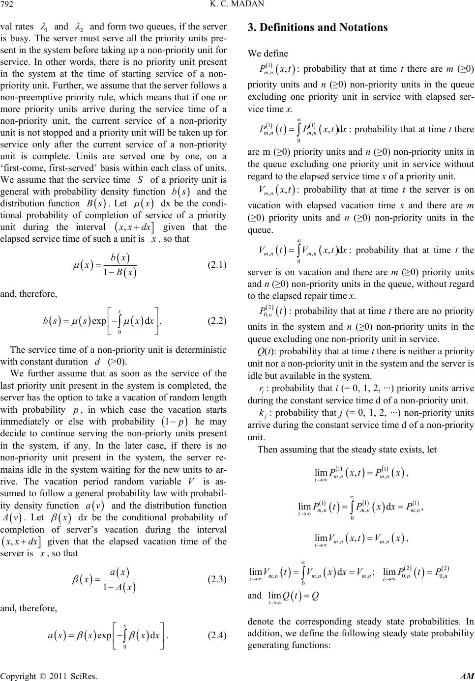 K. C. MADAN 792 val rates 1 and 2 and form two queues, if the server is busy. The server must serve all the priority units pre- sent in the system before taking up a non-priority unit for service. In other words, there is no priority unit present in the system at the time of starting service of a non- priority unit. Further, we assume that the server follows a non-preemptive priority rule, which means that if one or more priority units arrive during the service time of a non-priority unit, the current service of a non-priority unit is not stopped and a priority unit will be taken up for service only after the current service of a non-priority unit is complete. Units are served one by one, on a ‘first-come, first-served’ basis within each class of units. We assume that the service time of a priority unit is general with probability density function and the distribution function . Let S bs Bs dx be the condi- tional probability of completion of service of a priority unit during the interval , xdx given that the elapsed service time of such a unit is , so that 1 bx xBx (2.1) and, therefore, 0 expd . s bssx x (2.2) The service time of a non-priority unit is deterministic with constant duration (>0). d We further assume that as soon as the service of the last priority unit present in the system is completed, the server has the option to take a vacation of random length with probability , in which case the vacation starts immediately or else with probability he may decide to continue serving the non-priorty units present in the system, if any. In the later case, if there is no non-priority unit present in the system, the server re- mains idle in the system waiting for the new units to ar- rive. The vacation period random variable V is as- sumed to follow a general probability law with probabil- ity density function and the distribution function p 1p av v. Let dx be the conditional probability of completion of server’s vacation during the interval , xdx given that the elapsed vacation time of the server is , so that 1 ax x x (2.3) and, therefore, 0 exp d s assx x 3. Definitions and Notations . (2.4) We define 1 ,, mn Pxt: probability that at time t there are m (≥0) priority units and n (≥0) non-priority units in the queue excluding one priority unit in service with elapsed ser- vice time x. 11 ,, 0 ,d mn mn Pt Pxtx : probability that at time t there are m (≥0) priority units and n (≥0) non-priority units in the queue excluding one priority unit in service without regard to the elapsed service time x of a priority unit. ,, mn Vxt: probability that at time t the server is on vacation with elapsed vacation time x and there are m (≥0) priority units and n (≥0) non-priority units in the queue. ,, 0 ,d mn mn Vt Vxt x: probability that at time t the server is on vacation and there are m (≥0) priority units and n (≥0) non-priority units in the queue, without regard to the elapsed repair time x. 2 0,n t: probability that at time t there are no priority units in the system and n (≥0) non-priority units in the queue excluding one non-priority unit in service. Q(t): probability that at time t there is neither a priority unit nor a non-priority unit in the system and the server is idle but available in the system. i: probability that i (= 0, 1, 2, ···) priority units arrive during the constant service time d of a non-priority unit. r k: probability that j (= 0, 1, 2, ···) non-priority units arrive during the constant service time d of a non-priority unit. Then assuming that the steady state exists, let 11 ,, lim , mn mn tPxtPx , 11 ,, 0 limd , mn mnmn tPt PxxP 1 , ,, lim , mn mn tVxtVx 22 , ,, 0 limd ; mn mnmn tVt VxxV , 0, 0, lim nn tPtP and lim tQt Q denote the corresponding steady state probabilities. In addition, we define the following steady state probability enerating functions: g Copyright © 2011 SciRes. AM 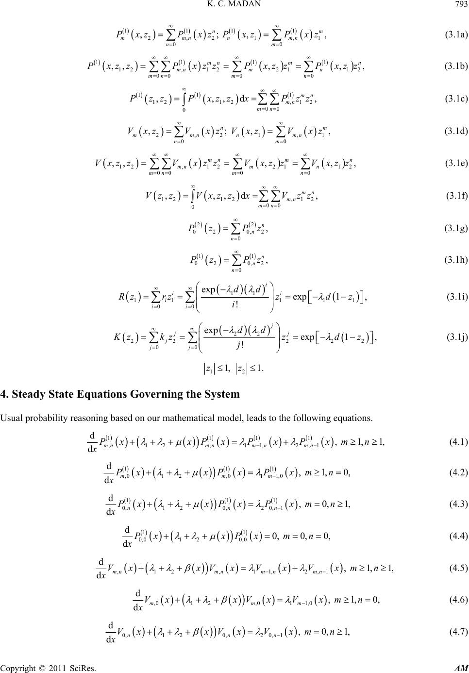 K. C. MADAN Copyright © 2011 SciRes. AM 793 1 , m , 1 , m , 2 1 1111 2,21 , 00 ,; , n mmnn mn nm PxzPxzPxz Pxz (3.1a) 1111 12, 122112 000 0 ,,,,, mnm n mn mn mn mn PxzzPxzz PxzzPxzz (3.1b) 11 1 12 12,12 00 0 ,,,d mn mn mn Pzz PxzzxPzz (3.1c) 2,21 , 00 ,; , n mmnn mn nm VxzV xzVxzV xz (3.1d) 12, 122112 000 0 ,,,, , mnm n mn m n mnm n VxzzVxzz Vxzz Vxzz (3.1e) 12 12,12 00 0 ,,,d mn mn mn VzzVxzzxVzz (3.1f) 2 02 0,2 0 , n n n Pz Pz (3.1g) 1 02 0,2 0 , n n n Pz Pz (3.1h) 11 111 11 00 exp exp1, ! i ii i ii dd Rzrzzd z i (3.1i) 22 222 2 00 exp exp1 , ! j jj j jj dd Kzkzzd z j 2 (3.1j) 12 1, 1.zz 4. Steady State Equations Governing the System Usual probability reasoning based on our mathematical model, leads to the following equations. 1111 ,12 ,11,2,1 d, 1,1, dmnmnm nmn PxxPxP xP xmn x (4.1) 111 ,012,01 1,0 d, 1,0, dmmm PxxPxPxm n x (4.2) 111 0,120,2 0,1 d, 0,1, dnnn PxxPxPxm n x (4.3) 11 0,0120,0 d0, 0,0, dPxxPxmn x (4.4) ,12 ,11,2,1 d, 1,1, dmnmnm nmn VxxVxV xV xmn x (4.5) ,012,01 1,0 d, 1,0, dmmm VxxVx Vxmn x (4.6) 0,120,20,1 d, 0,1, dnnn VxxVxVxm n x (4.7) 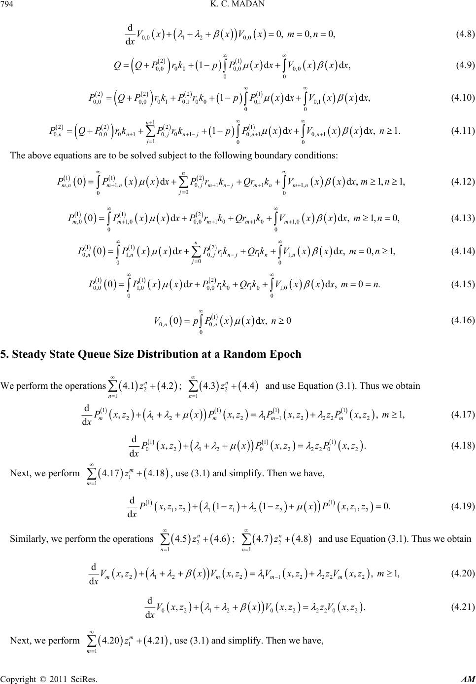 K. C. MADAN 794 0,01 20,0 d0, 0,0, dVxxVxm n x (4.8) 21 0,00 00,00,0 00 1dQQPrkpPxxVx xx d, d, ,1. 1,1, 1,0, 0,1, 0. n (4.9) 2221 0,00,0010,1000,10,1 00 1dPQPrk PrkpPxxVxxx (4.10) 1 22 21 0,0,0010,0 10,10,1 100 1dd n nnjnjnn j PQPrkPrkpPxxVxxxn (4.11) The above equations are to be solved subject to the following boundary conditions: 11 2 ,1, 0,111, 0 00 0dd, n mnmnjm njm nmn j PPxxxPrkQrkVxxxmn (4.12) 11 2 ,01,00,0 10101,0 00 0dd, mm mmm PPxxxPrkQrkVxxxmn (4.13) 11 2 0,1,0, 111, 0 00 0dd, n nn jnjnn j PPxxxPrkQrkVxxxmn (4.14) 11 2 0,01,00,010101,0 00 0dd, PPxxxPrkQrkVxxxm (4.15) 1 0, 0, 0 0 nn VpPxxxn d,0 (4.16) 5. Steady State Queue Size Distribution at a Random Epoch We perform the operations; and use Equation (3.1). Thus we obtain 2 1 4.1 4.2 n n z 2 1 4.3 4.4 n n z 1111 212211222 2 d,,, dmmmm PxzxPxzPxzzPxzm x ,, 1, (4.17) 11 0212 022202 d,, dPxzxPxz zPxz x 1 ,. (4.18) Next, we perform , use (3.1) and simplify. Then we have, 1 1 4.17 4.18 m m z 11 12112212 d,,11,,0. dPxzzzzxPxzz x (4.19) Similarly, we perform the operations ; and use Equation (3.1). Thus we obtain 2 1 4.5 4.6 n n z 2 1 4.7 4.8 n n z 212211222 2 d,,, dmmmm VxzxVxzVxzzVxz m x ,, 1, (4.20) 0212022202 d,, dVxzxVxz zVxz x ,. (4.21) Next, we perform , use (3.1) and simplify. Then we have, 1 1 4.20 4.21 m m z Copyright © 2011 SciRes. AM 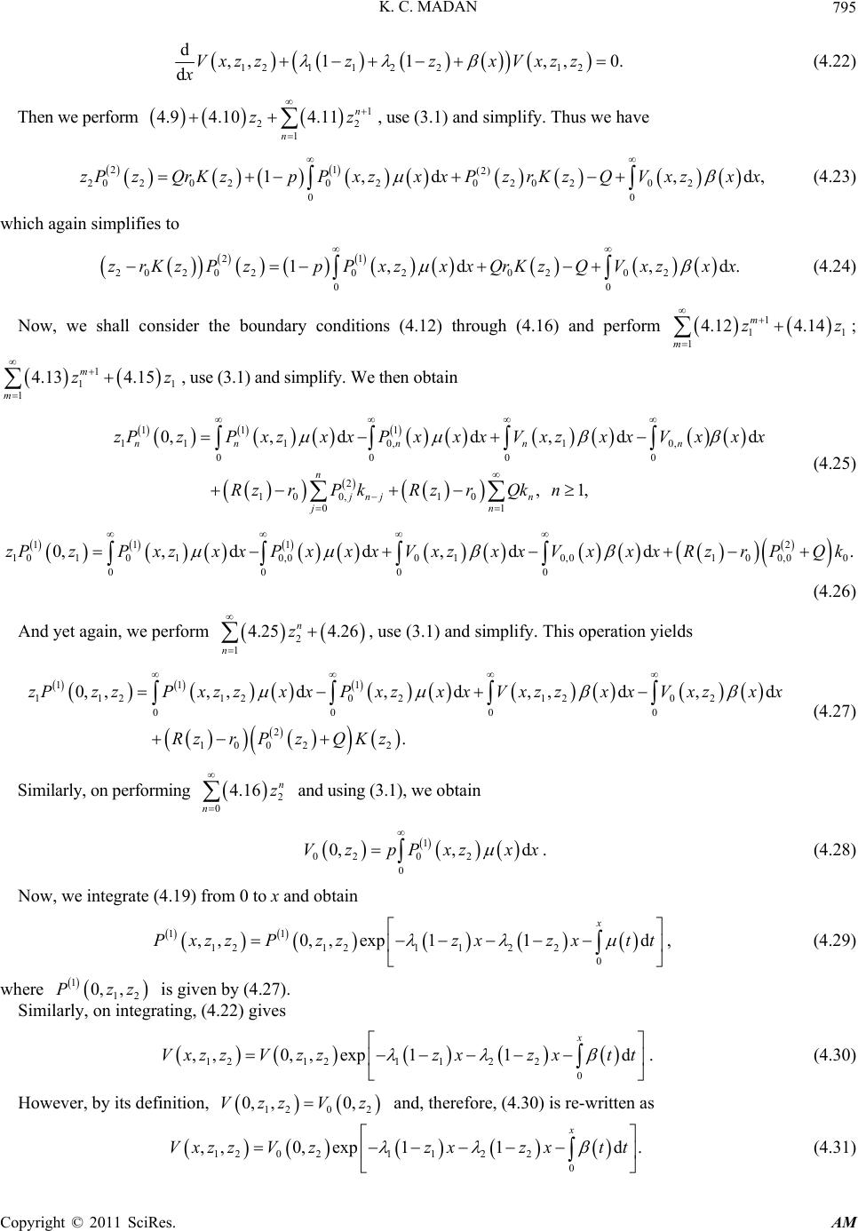 K. C. MADAN795 12112212 d,,11,, 0. dVxzzzzxVxzz x (4.22) Then we perform 1 2 1 4.94.104.11n n z 2 z , use (3.1) and simplify. Thus we have 21 (2) 2020 202020 202 00 1,d ,zPzQrK zpPxzxxPzrK zQVxzxx d, d. 1 z d x (4.23) which again simplifies to 21 20 202020 202 00 1,d ,zrKzPzpPxzxx QrKzQVxzxx (4.24) Now, we shall consider the boundary conditions (4.12) through (4.16) and perform ; , use (3.1) and simplify. We then obtain 1 11 1 4.12 4.14 m m zz 1 1 1 4.13 4.15 m m z 11 1 11 10,10, 0000 2 10 0,10 01 0,, dd, dd , 1, nnn nn n jnj n jn zPzP xzxxPxxxVxzxx Vxxx Rz rPkRzrQkn (4.25) 11 12 101010,0010,010 0,00 0000 0,, dd, dd.zPzPxzxxPxxxVxzx xVxx xRzrPQk (4.26) And yet again, we perform , use (3.1) and simplify. This operation yields 2 1 4.25 4.26 n n z 11 1 112 12021202 0000 2 100 22 0,,,,d,d,,d , . zPzzPxzzx xPxzx xVxzzx xVxzx x Rzr PzQKz (4.27) Similarly, on performing and using (3.1), we obtain 2 0 4.16 n n z 1 020 2 0 0,, dVz pPxzx . (4.28) Now, we integrate (4.19) from 0 to x and obtain 11 12121122 0 ,,0,, exp11d x Pxzz Pzzzxzxtt , (4.29) where is given by (4.27). 1 12 0, ,Pzz Similarly, on integrating, (4.22) gives 12121 122 0 ,,0,,exp11d x VxzzVzzz xzxtt . (4.30) However, by its definition, and, therefore, (4.30) is re-written as 120 2 0, ,0,VzzV z 120 21122 0 ,,0,exp11d. x VxzzVzz xzxtt (4.31) Copyright © 2011 SciRes. AM 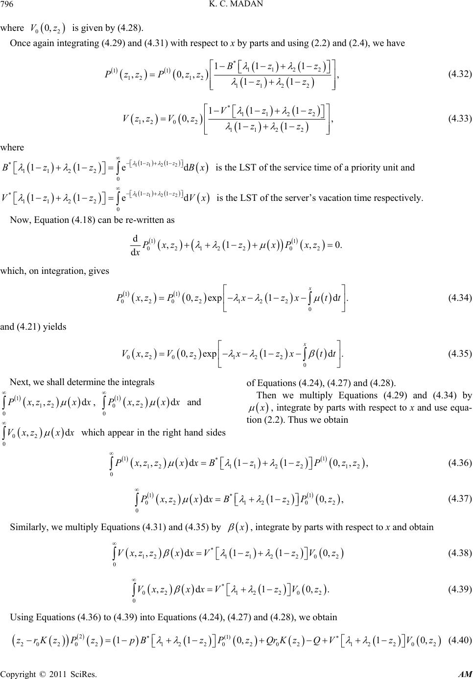 K. C. MADAN Copyright © 2011 SciRes. AM 796 where is given by (4.28). 02 0,Vz Once again integrating (4.29) and (4.31) with respect to x by parts and using (2.2) and (2.4), we have * 112 2 11 12 12 112 2 111 ,0,,11 Bzz Pzz Pzzzz , (4.32) * 112 2 120 2 112 2 111 ,0, 11 Vz z Vzz V zzz , (4.33) where 1122 11 * 112 2 0 11ed zz Bz zB 1122 11 * 112 2 0 11ed zz Vz zV x x is the LST of the service time of a priority unit and is the LST of the server’s vacation time respectively. Now, Equation (4.18) can be re-written as 11 02122 02 d,1 , dPxzzxPxz x 0. d. which, on integration, gives 11 0202 122 0 ,0,exp 1 x PxzPzxzxtt (4.34) and (4.21) yields 0202122 0 ,0,exp 1 x VxzV zxzxtt d. (4.35) Next, we shall determine the integrals of Equations (4.24), (4.27) and (4.28). 1 12 0 ,, dPxzz xx , and 1 02 0 ,Pxz xx Then we multiply Equations (4.29) and (4.34) by , integrate by parts with respect to x and use equa- tion (2.2). Thus we obtain d d 02 0 ,Vxz xx which appear in the right hand sides 1 1 * 1211 2212 0 ,,d110,, ,Pxzzx xBzzPzz 1 , (4.36) 1 * 02 12202 0 ,d1 0,PxzxxBzPz (4.37) Similarly, we multiply Equations (4.31) and (4.35) by , integrate by parts with respect to x and obtain * 12112202 0 ,, d110,Vxzzx x VzzVz . 0, (4.38) * 0212202 0 ,d10,VxzxxVzVz (4.39) Using Equations (4.36) to (4.39) into Equations (4.24), (4.27) and (4.28), we obtain 2(1) 2020212202021 2202 110,1zrKzPzpBzPz QrKz QVzVz (4.40) 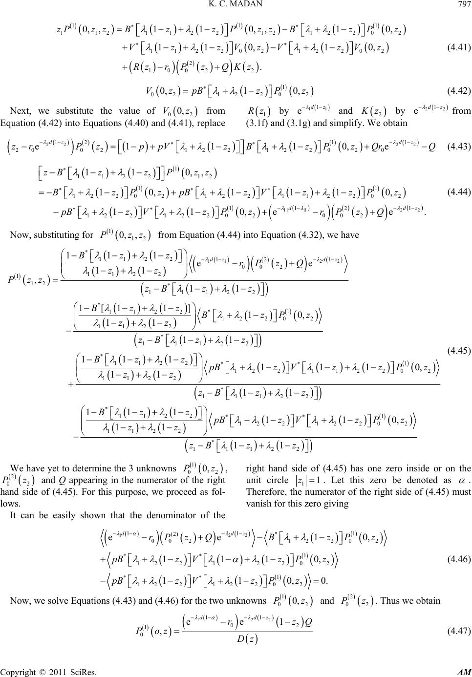 K. C. MADAN797 1 2 , 11 112112212 1220 112 20212 202 2 100 22 0,,110,,10 110,10, . zP zzBzzPzzBzPz VzzV zVzVz Rzr PzQKz (4.41) 1 0212202 0,1 0,Vz pBzPz (4.42) Next, we substitute the value of 02 0,Vz from Equation (4.42) into Equations (4.40) and (4.41), replace 1 Rz by and 11 edz 1 2 z by from (3.1f) and (3.1g) and simplify. We obtain 22 1 edz 1 1 z 22 22 12 1 20021 221 22020 e1110,e dz dz zrPzppVzBzPzQrQ (4.43) 11 1122 1 112 212 1 1 1220 212211220 2 112 12 212 202002 11 0,, 10,1 110, 110,ee. dd zBzzPzz BzPzpBzVzzPz pBzVzPzr PzQ 1 (4.44) Now, substituting for from Equation (4.44) into Equation (4.32), we have 12 0, ,Pzz 112 2 * 112 212 1 00 2 112 2 1 12 * 11122 * 1 112 2* 12 202 112 2 * 1112 111 ee 11 ,11 1[11]10, 11 1 dz dz Bz zrP zQ zz Pzz zB zz Bz z BzPz zz zB z 2 * 112 21 ** 12 2112 202 112 2 * 11122 * 112 2 112 2 1 11 11110 11 11 111 11 z Bzz pBz VzzPz zz zB zz Bzz zz , 1 ** 12 212 202 * 11122 110, 11 pBz VzPz zB zz (4.45) We have yet to determine the 3 unknowns , and Q appearing in the numerator of the right hand side of (4.45). For this purpose, we proceed as fol- lows. 1 02 0,Pz 2 02 Pz It can be easily shown that the denominator of the right hand side of (4.45) has one zero inside or on the unit circle 11z . Let this zero be denoted as . Therefore, the numerator of the right side of (4.45) must vanish for this zero giving 122 11 (2) * 00212202 1 ** 12 212 202 1 ** 12 212202 ee1 1110, 110,0. ddz rPzQBz Pz pBz VzPz pBz VzPz 1 0, 2 (4.46) Now, we solve Equations (4.43) and (4.46) for the two unknowns and . Thus we obtain 1 0 0,Pz 2 02 Pz 122 11 0 1 0 ee1 , ddz rz Poz Dz 2 Q (4.47) Copyright © 2011 SciRes. AM 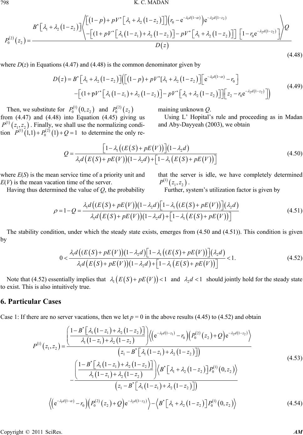 K. C. MADAN 798 122 22 11 122 0 12 21 112 212 20 2 02 11ee 1 (1111 1e ddz dz ppVz r Bz Q pVzzpVzr Pz Dz (4.48) where D(z) in Equations (4.47) and (4.48) is the common denominator given by 1 22 1 12 212 20 1 112 212 220 11 [1e (1p111e d dz DzBzp pVzr Vz zpVzzr (4.49) Then, we substitute for and 1 0 0,Pz 2 from (4.47) and (4.48) into Equation (4.45) giving us . Finally, we shall use the normalizing condi- tion to determine the only re- 2 02 Pz 1 12 ,Pzz 1,1 12 011PPQ maining unknown Q. Using L’ Hopital’s rule and proceeding as in Madan and Aby-Dayyeah (2003), we obtain 12 121 1( 1 11 ES pEVd QdESpEVdESpEV (4.50) where E(S) is the mean service time of a priority unit and E(V) is the mean vacation time of the server. Having thus determined the value of Q, the probability that the server is idle, we have completely determined . 1 12 ,Pzz Further, system’s utilization factor is given by 121 121 (11( 111 dESpEVdESpEV d QdESpEV dESpEV 2 (4.51) The stability condition, under which the steady state exists, emerges from (4.50 and (4.51)). This condition is given by 121 121 (11( 01 11 d ESpEVdESpEVd dESpEVdESpEV 2 . (4.52) Note that (4.52) essentially implies that 11ESpEV and 21d should jointly hold for the steady state to exist. This is also intuitively true. 6. Particular Cases Case 1: If there are no server vacations, then we let p = 0 in the above results (4.45) to (4.52) and obtain 112 2 * 112 212 1 00 2 112 2 1 12 * 11122 * 112 21 * 12 202 112 2 * 111 111ee 11 ,11 11 110, 11 1 dz dz Bz zrP zQ zz Pzz zB zz Bzz BzPz zz zB z 22 1z (4.53) 122 12 11 * 002122 02 ee1 ddz rPzQBz Pz 0, (4.54) Copyright © 2011 SciRes. AM 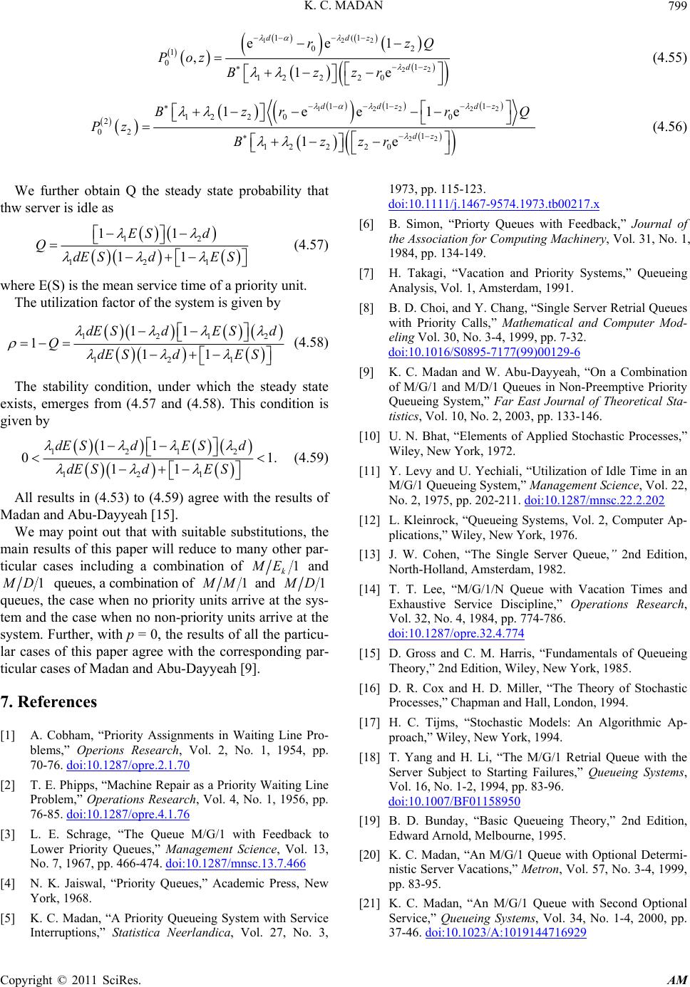 K. C. MADAN799 122 22 1(1 0 1 01 12 220 ee1 , 1e ddz dz rz PozBzzr 2 Q (4.55) 122 22 22 11 1 122 00 2 02 1 12 220 1ee1e 1e ddz dz dz Bzr r Pz Bzzr Q (4.56) We further obtain Q the steady state probability that thw server is idle as 12 121 11 11 ES d QdESdES (4.57) where E(S) is the mean service time of a priority unit. The utilization factor of the system is given by 121 121 11 111 dE SdE Sd QdE SdES 2 (4.58) The stability condition, under which the steady state exists, emerges from (4.57 and (4.58). This condition is given by 1212 121 11 0 11 dE SdE Sd dE SdES 1. (4.59) All results in (4.53) to (4.59) agree with the results of Madan and Abu-Dayyeah [15]. We may point out that with suitable substitutions, the main results of this paper will reduce to many other par- ticular cases including a combination of 1 k E and 1 D queues, a combination of 1 M and 1 D queues, the case when no priority units arrive at the sys- tem and the case when no non-priority units arrive at the system. Further, with p = 0, the results of all the particu- lar cases of this paper agree with the corresponding par- ticular cases of Madan and Abu-Dayyeah [9]. 7. References [1] A. Cobham, “Priority Assignments in Waiting Line Pro- blems,” Operions Research, Vol. 2, No. 1, 1954, pp. 70-76. doi:10.1287/opre.2.1.70 [2] T. E. Phipps, “Machine Repair as a Priority Waiting Line Problem,” Operations Research, Vol. 4, No. 1, 1956, pp. 76-85. doi:10.1287/opre.4.1.76 [3] L. E. Schrage, “The Queue M/G/1 with Feedback to Lower Priority Queues,” Management Science, Vol. 13, No. 7, 1967, pp. 466-474. doi:10.1287/mnsc.13.7.466 [4] N. K. Jaiswal, “Priority Queues,” Academic Press, New York, 1968. [5] K. C. Madan, “A Priority Queueing System with Service Interruptions,” Statistica Neerlandica, Vol. 27, No. 3, 1973, pp. 115-123. doi:10.1111/j.1467-9574.1973.tb00217.x [6] B. Simon, “Priorty Queues with Feedback,” Journal of the Association for Computing Machinery, Vol. 31, No. 1, 1984, pp. 134-149. [7] H. Takagi, “Vacation and Priority Systems,” Queueing Analysis, Vol. 1, Amsterdam, 1991. [8] B. D. Choi, and Y. Chang, “Single Server Retrial Queues with Priority Calls,” Mathematical and Computer Mod- eling Vol. 30, No. 3-4, 1999, pp. 7-32. doi:10.1016/S0895-7177(99)00129-6 [9] K. C. Madan and W. Abu-Dayyeah, “On a Combination of M/G/1 and M/D/1 Queues in Non-Preemptive Priority Queueing System,” Far East Journal of Theoretical Sta- tistics, Vol. 10, No. 2, 2003, pp. 133-146. [10] U. N. Bhat, “Elements of Applied Stochastic Processes,” Wiley, New York, 1972. [11] Y. Levy and U. Yechiali, “Utilization of Idle Time in an M/G/1 Queueing System,” Management Science, Vol. 22, No. 2, 1975, pp. 202-211. doi:10.1287/mnsc.22.2.202 [12] L. Kleinrock, “Queueing Systems, Vol. 2, Computer Ap- plications,” Wiley, New York, 1976. [13] J. W. Cohen, “The Single Server Queue,” 2nd Edition, North-Holland, Amsterdam, 1982. [14] T. T. Lee, “M/G/1/N Queue with Vacation Times and Exhaustive Service Discipline,” Operations Research, Vol. 32, No. 4, 1984, pp. 774-786. doi:10.1287/opre.32.4.774 [15] D. Gross and C. M. Harris, “Fundamentals of Queueing Theory,” 2nd Edition, Wiley, New York, 1985. [16] D. R. Cox and H. D. Miller, “The Theory of Stochastic Processes,” Chapman and Hall, London, 1994. [17] H. C. Tijms, “Stochastic Models: An Algorithmic Ap- proach,” Wiley, New York, 1994. [18] T. Yang and H. Li, “The M/G/1 Retrial Queue with the Server Subject to Starting Failures,” Queueing Systems, Vol. 16, No. 1-2, 1994, pp. 83-96. doi:10.1007/BF01158950 [19] B. D. Bunday, “Basic Queueing Theory,” 2nd Edition, Edward Arnold, Melbourne, 1995. [20] K. C. Madan, “An M/G/1 Queue with Optional Determi- nistic Server Vacations,” Metron, Vol. 57, No. 3-4, 1999, pp. 83-95. [21] K. C. Madan, “An M/G/1 Queue with Second Optional Service,” Queueing Systems, Vol. 34, No. 1-4, 2000, pp. 37-46. doi:10.1023/A:1019144716929 Copyright © 2011 SciRes. AM
|