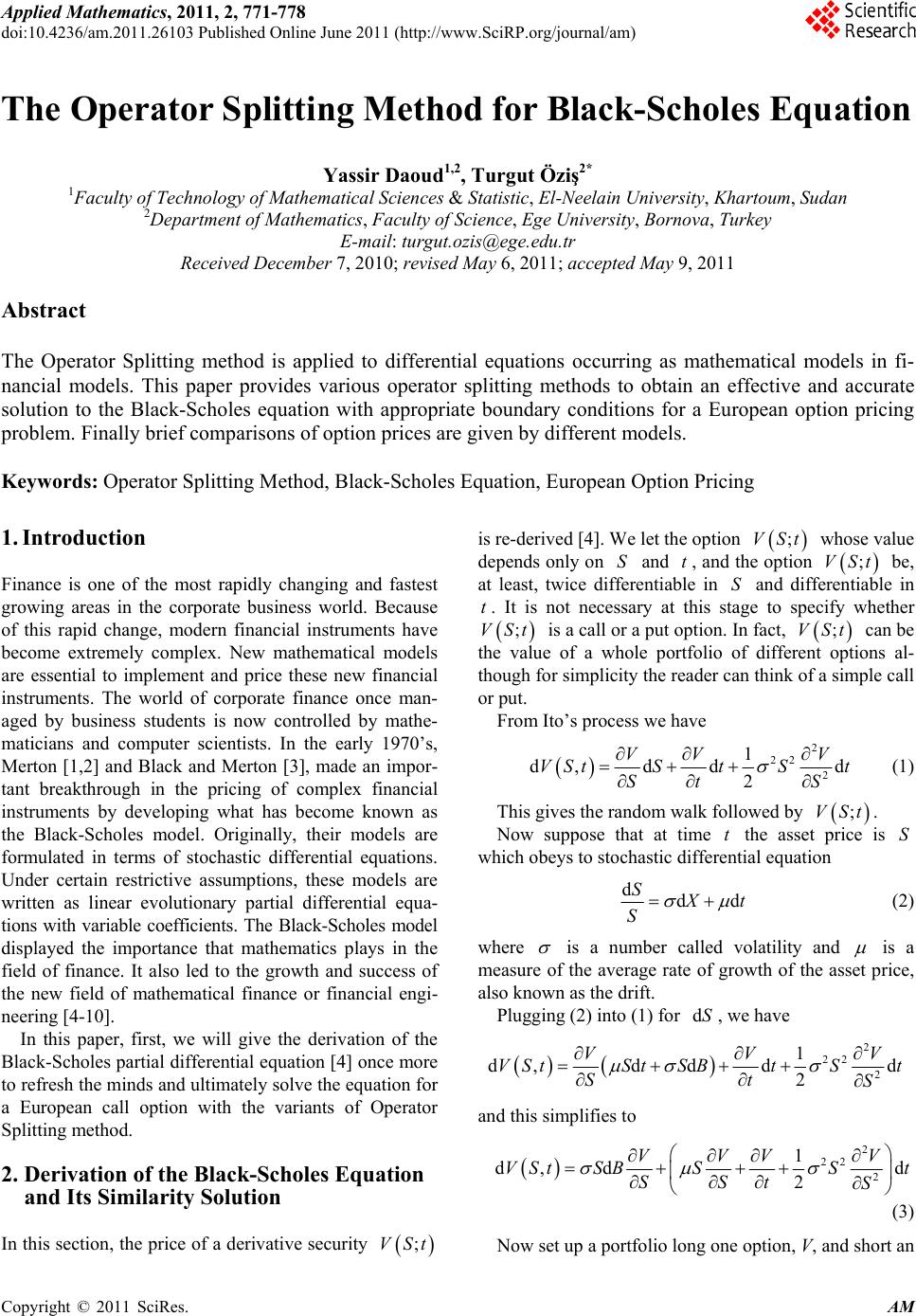
Applied Mathematics, 2011, 2, 771-778
doi:10.4236/am.2011.26103 Published Online June 2011 (http://www.SciRP.org/journal/am)
The Operator Splitting Method for Black-Scholes Equation
Yassir Daoud1,2, Turgut Öziş2*
1Faculty of Technology of M at hem at i cal Sci ences & Statistic, El-Neelain University, Khartoum, Sudan
2Department of Mat hem at i cs, Faculty of Science, Ege University, Bornova, Turkey
Received December 7, 2010; revised May 6, 2011; accepted May 9, 2011
Abstract
The Operator Splitting method is applied to differential equations occurring as mathematical models in fi-
nancial models. This paper provides various operator splitting methods to obtain an effective and accurate
solution to the Black-Scholes equation with appropriate boundary conditions for a European option pricing
problem. Finally brief comparisons of option prices are given by different models.
Keywords: Operator Splitting Method, Black-Scholes Equation, European Option Pricing
1. Introduction
Finance is one of the most rapidly changing and fastest
growing areas in the corporate business world. Because
of this rapid change, modern financial instruments have
become extremely complex. New mathematical models
are essential to implement and price these new financial
instruments. The world of corporate finance once man-
aged by business students is now controlled by mathe-
maticians and computer scientists. In the early 1970’s,
Merton [1,2] and Black and Merton [3], made an impor-
tant breakthrough in the pricing of complex financial
instruments by developing what has become known as
the Black-Scholes model. Originally, their models are
formulated in terms of stochastic differential equations.
Under certain restrictive assumptions, these models are
written as linear evolutionary partial differential equa-
tions with variable coefficients. The Black-Scholes model
displayed the importance that mathematics plays in the
field of finance. It also led to the growth and success of
the new field of mathematical finance or financial engi-
neering [4-10].
In this paper, first, we will give the derivation of the
Black-Scholes partial differential equation [4] once more
to refresh the minds and ultimately solve the equation for
a European call option with the variants of Operator
Splitting method.
2. Derivation of the Black-Scholes Equation
and Its Similarity Solution
In this section, the price of a derivative security


;VSt
is re-derived [4]. We let the option


;VSt whose value
depends only on and t, and the option S


;VSt be,
at least, twice differentiable in and differentiable in
. It is not necessary at this stage to specify whether
S
t


;VSt is a call or a put option. In fact, can be
the value of a whole portfolio of different options al-
though for simplicity the reader can think of a simple call
or put.

;VSt
From Ito’s process we have

2
22
1
2SS

2d
V
t

d, dVStSdt
VV
St

 (1)
This gives the random walk followed by


;VSt.
Now suppose that at time the asset price is
which obeys to stochastic differential equation
t S
dSdd
X
t
S

  (2)
where

is a number called volatility and

is a
measure of the average rate of growth of the asset price,
also known as the drift.
Plugging (2) into (1) for , we have
dS
 
2
22
2
1
d ddd
2
V
tt BtSt
S
 



d,VS VV
St


S S
and this simplifies to

2
22
2
1
d,
VS d Bd
2
VVV V
t SSSt
SSt S

  


 


(3)
Now set up a portfolio long one option, V, and short an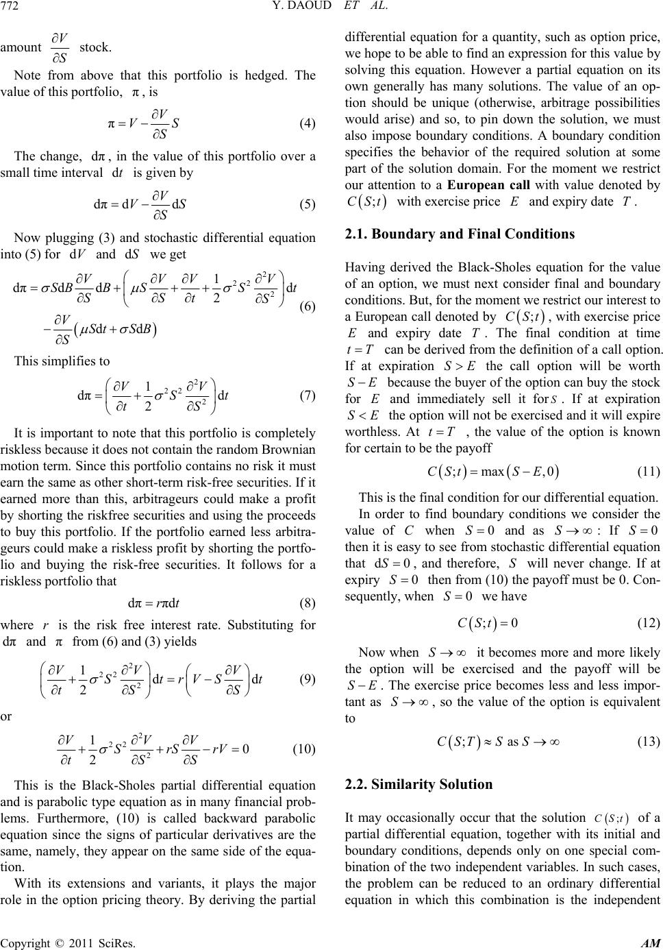

Y. DAOUD ET AL. 772
amount V
S

 stock.
Note from above that this portfolio is hedged. The
value of this portfolio, , is π
πV
V
S


S
(4)
The change, , in the value of this portfolio over a
small time interval is given by
dπ
dt
dπd
V
V
S


dS (5)
Now plugging (3) and stochastic differential equation
into (5) for and we get
dVdS

2
22
2
1
dπdd 2
dd
VVV
SBB SSt
SStS
VSt SB
S












d
V



(6)
This simplifies to
2
22
2
1
dπd
2
V
S
tS

 




V
t

(7)
It is important to note that this portfolio is completely
riskless because it does not contain the random Brownian
motion term. Since this portfolio contains no risk it must
earn the same as other short-term risk-free securities. If it
earned more than this, arbitrageurs could make a profit
by shorting the riskfree securities and using the proceeds
to buy this portfolio. If the portfolio earned less arbitra-
geurs could make a riskless profit by shorting the portfo-
lio and buying the risk-free securities. It follows for a
riskless portfolio that
dππdrt (8)
where is the risk free interest rate. Substituting for
and from (6) and (3) yields
r
dππ
2
22
2
1dd
2
VV
StrVS
t S

  







V
t
S



(9)
or
2
22
2
10
2
VVV
SrSrV
tS
S





(10)
This is the Black-Sholes partial differential equation
and is parabolic type equation as in many financial prob-
lems. Furthermore, (10) is called backward parabolic
equation since the signs of particular derivatives are the
same, namely, they appear on the same side of the equa-
tion.
With its extensions and variants, it plays the major
role in the option pricing theory. By deriving the partial
differential equation for a quantity, such as option price,
we hope to be able to find an expression for this value by
solving this equation. However a partial equation on its
own generally has many solutions. The value of an op-
tion should be unique (otherwise, arbitrage possibilities
would arise) and so, to pin down the solution, we must
also impose boundary conditions. A boundary condition
specifies the behavior of the required solution at some
part of the solution domain. For the moment we restrict
our attention to a European call with value denoted by


;CSt with exercise price and expiry date .
E T
2.1. Boundary and Final Conditions
Having derived the Black-Sholes equation for the value
of an option, we must next consider final and boundary
conditions. But, for the moment we restrict our interest to
a European call denoted by , with exercise price
and expiry date T. The final condition at time

;CSt
E
tT

can be derived from the definition of a call option.
If at expiration the call option will be worth
SE
SE

because the buyer of the option can buy the stock
for and immediately sell it for. If at expiration ES
SE

the option will not be exercised and it will expire
worthless. At tT

, the value of the option is known
for certain to be the payoff


;max ,0CStS E

(11)
This is the final condition for our differential equation.
In order to find boundary conditions we consider the
value of C when 0S

and as : If S 0S

then it is easy to see from stochastic differential equation
that dS0

, and therefore, will never change. If at
expiry
S
0S

then from (10) the payoff must be 0. Con-
sequently, when 0S

we have


;CSt0 (12)
Now when it becomes more and more likely
the option will be exercised and the payoff will be
S
SE

. The exercise price becomes less and less impor-
tant as , so the value of the option is equivalent
to
S


; as CSTSS

 (13)
2.2. Similarity Solution
It may occasionally occur that the solution


;CSt of a
partial differential equation, together with its initial and
boundary conditions, depends only on one special com-
bination of the two independent variables. In such cases,
the problem can be reduced to an ordinary differential
equation in which this combination is the independent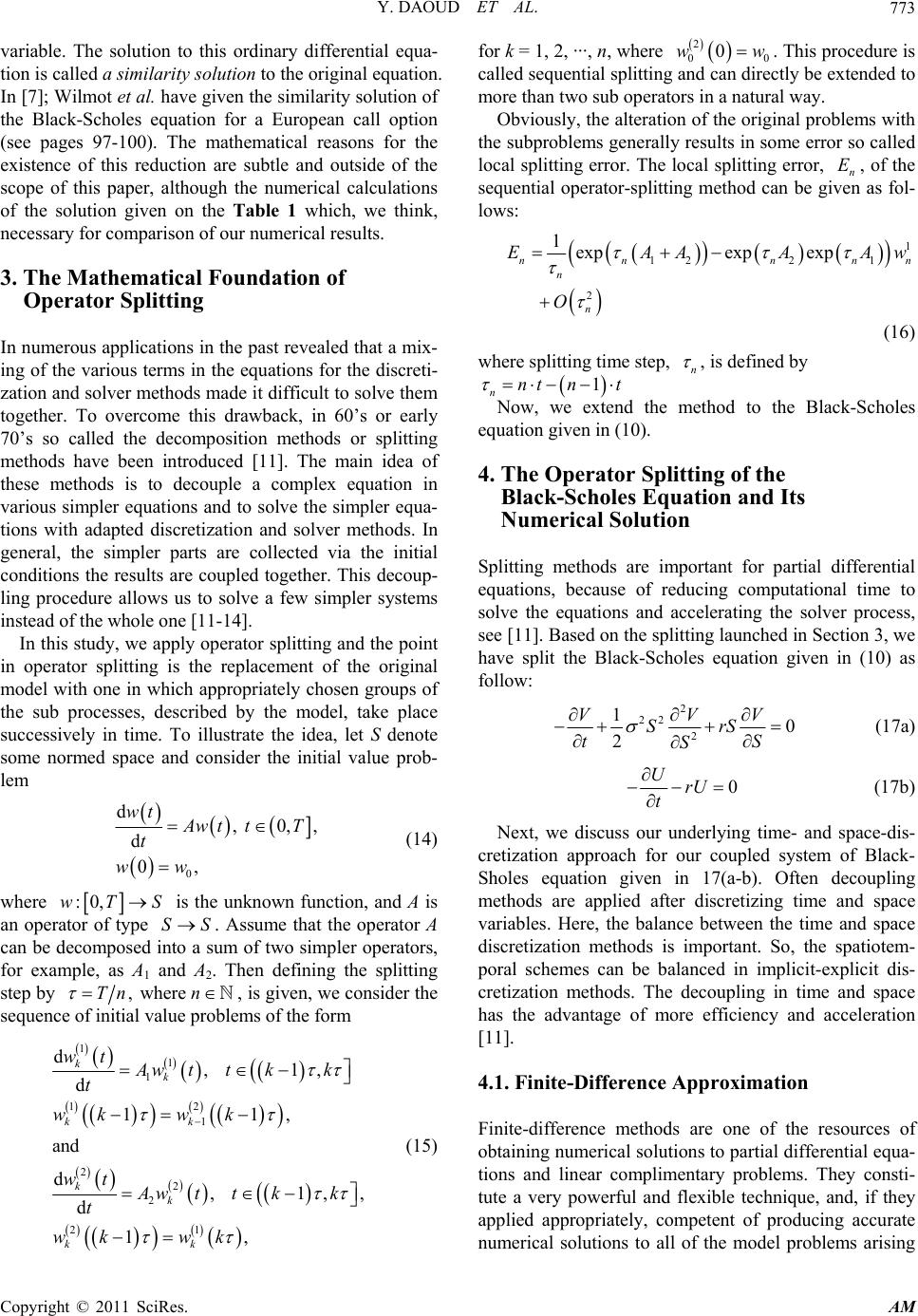

Y. DAOUD ET AL.773
variable. The solution to this ordinary differential equa-
tion is called a similarity solution to the original equation.
In [7]; Wilmot et al. have given the similarity solution of
the Black-Scholes equation for a European call option
(see pages 97-100). The mathematical reasons for the
existence of this reduction are subtle and outside of the
scope of this paper, although the numerical calculations
of the solution given on the Table 1 which, we think,
necessary for comparison of our numerical results.
3. The Mathematical Foundation of
Operator Splitting
In numerous applications in the past revealed that a mix-
ing of the various terms in the equations for the discreti-
zation and solver methods made it difficult to solve them
together. To overcome this drawback, in 60’s or early
70’s so called the decomposition methods or splitting
methods have been introduced [11]. The main idea of
these methods is to decouple a complex equation in
various simpler equations and to solve the simpler equa-
tions with adapted discretization and solver methods. In
general, the simpler parts are collected via the initial
conditions the results are coupled together. This decoup-
ling procedure allows us to solve a few simpler systems
instead of the whole one [11-14].
In this study, we apply operator splitting and the point
in operator splitting is the replacement of the original
model with one in which appropriately chosen groups of
the sub processes, described by the model, take place
successively in time. To illustrate the idea, let S denote
some normed space and consider the initial value prob-
lem
  


0
d, 0,,
d
0,
wt
A
wt tT
t
ww


(14)
where


:0,wTSS is the unknown function, and A is
an operator of type . Assume that the operator A
can be decomposed into a sum of two simpler operators,
for example, as A1 and A2. Then defining the splitting
step by
S
, where Tn n

, is given, we consider the
sequence of initial value problems of the form



 


 

 



 

 


1
1
1
12
1
2
2
2
21
d, 1,
d
11,
and
d, 1,,
d
1,
kk
kk
kk
kk
wt Aw ttkk
t
wkw k
wt Aw ttkk
t
wk wk









 





w
(15)
for k = 1, 2, ···, n, where 0
. This procedure is
called sequential splitting and can directly be extended to
more than two sub operators in a natural way.


2
0
0w
Obviously, the alteration of the original problems with
the subproblems generally results in some error so called
local splitting error. The local splitting error, n, of the
sequential operator-splitting method can be given as fol-
lows:
E
 



1
122 1
2
1expexp exp
nn nn
n
n
EAAA
O





n
Aw
(16)
where splitting time step, n

, is defined by


1
nnt nt


 
Now, we extend the method to the Black-Scholes
equation given in (10).
4. The Operator Splitting of the
Black-Scholes Equation and Its
Numerical Solution
Splitting methods are important for partial differential
equations, because of reducing computational time to
solve the equations and accelerating the solver process,
see [11]. Based on the splitting launched in Section 3, we
have split the Black-Scholes equation given in (10) as
follow:
2
22
2
10
2
VVV
SrS
tS S







(17a)
0
UrU
t



 (17b)
Next, we discuss our underlying time- and space-dis-
cretization approach for our coupled system of Black-
Sholes equation given in 17(a-b). Often decoupling
methods are applied after discretizing time and space
variables. Here, the balance between the time and space
discretization methods is important. So, the spatiotem-
poral schemes can be balanced in implicit-explicit dis-
cretization methods. The decoupling in time and space
has the advantage of more efficiency and acceleration
[11].
4.1. Finite-Difference Approximation
Finite-difference methods are one of the resources of
obtaining numerical solutions to partial differential equa-
tions and linear complimentary problems. They consti-
tute a very powerful and flexible technique, and, if they
applied appropriately, competent of producing accurate
numerical solutions to all of the model problems arising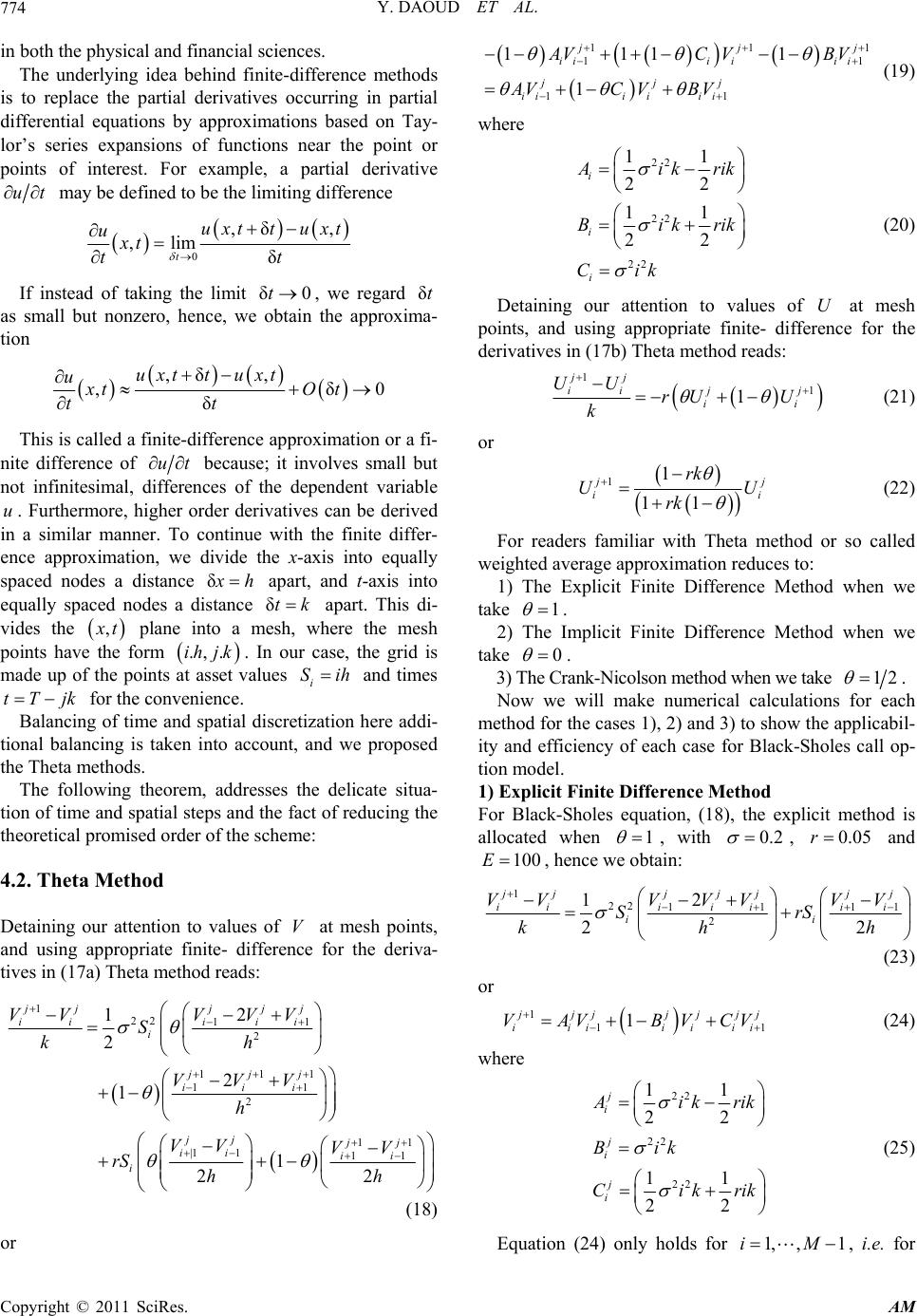

Y. DAOUD ET AL. 774
in both the physical and financial sciences.
The underlying idea behind finite-difference methods
is to replace the partial derivatives occurring in partial
differential equations by approximations based on Tay-
lor’s series expansions of functions near the point or
points of interest. For example, a partial derivative
ut may be defined to be the limiting difference
 
0
,δ,
,lim δ
t
uxttuxt
uxt
tt
 



If instead of taking the limit , we regard
as small but nonzero, hence, we obtain the approxima-
tion
δ0tδt
  
,δ,
,δ0
δ
uxttuxt
uxtO t
tt



This is called a finite-difference approximation or a fi-
nite difference of ut because; it involves small but
not infinitesimal, differences of the dependent variable
. Furthermore, higher order derivatives can be derived
in a similar manner. To continue with the finite differ-
ence approximation, we divide the x-axis into equally
spaced nodes a distance
u
δ
x
h

apart, and t-axis into
equally spaced nodes a distance apart. This di-
vides the

δtk

,
x
t
k
plane into a mesh, where the mesh
points have the form . In our case, the grid is
made up of the points at asset values and times
for the convenience.

., .jkih
i
Sih
tT j
Balancing of time and spatial discretization here addi-
tional balancing is taken into account, and we proposed
the Theta methods.
The following theorem, addresses the delicate situa-
tion of time and spatial steps and the fact of reducing the
theoretical promised order of the scheme:
4.2. Theta Method
Detaining our attention to values of at mesh points,
and using appropriate finite- difference for the deriva-
tives in (17a) Theta method reads:
V


1
22 11
2
111
11
2
11
|1 111
2
1
2
2
1
1
22
jjj jj
iii ii
i
jjj
iii
jj jj
ii ii
i
VV VVV
S
kh
VVV
h
VV VV
rS hh








 








 








 







(18)
or








11
11
11
1111
1
1
j
jj
iii iii
jjj
iii iii
A
VCV
AVC VBV


BV





 
  (19)
where
22
22
22
11
22
11
22
i
i
i
A
ik rik
Bikr
Cik












ik


(20)
Detaining our attention to values of U at mesh
points, and using appropriate finite- difference for the
derivatives in (17b) Theta method reads:


1
1
1
jj j
ii i
UU rU U
k


j
i
(21)
or


 
11
11
j
j
i
rk
U
rk



 i U (22)
For readers familiar with Theta method or so called
weighted average approximation reduces to:
1) The Explicit Finite Difference Method when we
take 1


.
2) The Implicit Finite Difference Method when we
take 0


.
3) The Crank-Nicolson method when we take 12


.
Now we will make numerical calculations for each
method for the cases 1), 2) and 3) to show the applicabil-
ity and efficiency of each case for Black-Sholes call op-
tion model.
1) Explicit Finite Difference Method
For Black-Sholes equation, (18), the explicit method is
allocated when 1


, with 0.2

, and 0.05r
100E

, hence we obtain:
1
22 111
2
2
1
22
jjj jjjj
iii iiii
ii
VVVVV VV
SrS
kh h








1





(23)
or


1
1
11
j
jjj jjj
iii iii
VAV BVCV
i


  (24)
where
22
22
22
11
22
11
22
j
i
j
i
j
i
A
ik rik
Bik
Cikr












ik

(25)
Equation (24) only holds for , i.e. for 1, ,1iM 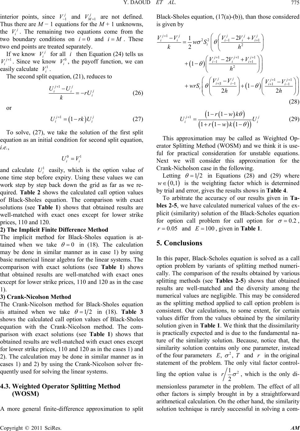

Y. DAOUD ET AL.775
interior points, since 1
j
V and 1
j
M
V are not defined.
Thus there are M − 1 equations for the M + 1 unknowns,
the
j
i
V. The remaining two equations come from the
two boundary conditions on and i. These
two end points are treated separately.
0iM
If we know
j
i
V for all i then Equation (24) tells us
1
j
i
V. Since we know , the payoff function, we can
easily calculate .
0
i
V
1
i
V
The second split equation, (21), reduces to
1jj
j
ii i
rU

UU
k

1


(26)
or
1
j
j
rk
i
 i U
U (27)
To solve, (27), we take the solution of the first split
equation as an initial condition for second split equation,
i.e.,
01
ii
UV
and calculate easily, which is the option value of
one time step before expiry. Using these values we can
work step by step back down the grid as far as we re-
quired. Table 2 shows the calculated call option values
of Black-Sholes equation. The comparison with exact
solutions (see Table 1) shows that obtained results are
well-matched with exact ones except for lower strike
prices, 110 and 120.
1
i
U
2) The Implicit Finite Difference Method
The implicit method for Black-Sholes equation is at-
tained when we take 0

 in (18). The calculation
may be done in similar manner as in case 1) by using
basic numerical linear algebra for the linear systems. The
comparison with exact solutions (see Table 1) shows
that obtained results are well-matched with exact ones
except for lower strike prices, 110 and 120 as in the case
1).
3) Crank-Nicolson Method
The Crank-Nicolson method for Black-Sholes equation
is attained when we take 12

 in (18). Table 3
shows the calculated call option values of Black-Sholes
equation with the Crank-Nicolson method. The com-
parison with exact solutions (see Table 1) shows that
obtained results are well-matched with exact ones except
for lower strike prices, 110 and 120 as in the cases 1) and
2). The calculation may be done in similar manner as in
cases 1) and 2) by using the Crank-Nicolson solver fre-
quently used for solving the linear systems.
4.3. Weighted Operator Splitting Method
(WOSM)
A more general finite-difference approximation to split
Black-Sholes equation, (17(a)-(b)), than those considered
is given by


1
22 11
2
111
11
2
11
|1 111
2 1
2
2
1
1
22
jjj jj
iii ii
i
jjj
iii
jj jj
ii ii
i
VV VVV
wS
kh
VVV
h
VV VV
wrS hh








 








 





















(28)




 
111
11 1
j
j
ii
rwk
UU
rwk



  (29)
This approximation may be called as Weighted Op-
erator Splitting Method (WOSM) and we think it is use-
ful for practical consideration for unstable equations.
Next we will consider this approximation for the
Crank-Nicholson case in the following.
Letting 12


in Equations (28) and (29) where


0, 1w is the weighting factor which is determined
by trial and error, gives the results shows in Table 4.
To arbitrate the accuracy of our results given in Ta-
bles 2-5, we have calculated numerical values of the ex-
plicit (similarity) solution of the Black-Scholes equation
for option call problem for call option for 0.2


,
0.05r

and 100E

, given in Table 1.
5. Conclusions
In this paper, Black-Scholes equation is solved as a call
option problem by variants of splitting method numeri-
cally. The comparison of the results obtained by various
splitting methods (see Tables 2-5) shows that obtained
results are well-matched and the diversity among the
numerical values are negligible. This may be considered
as the splitting method applied to call option problem is
consistent. Our calculations, to some extent, for certain
values differ from the values obtained by the similarity
solution given in Table 1. We think that the dissimilarity
is practically expected and is due to the fundamental na-
ture of the similarity solution. Because, notice that, the
similarity solution contains only one parameter, instead
of the four parameters and r in the original
statement of the problem. The only vital factor control-
2
, , E  T
ling the option value is 2
1
2
r

, which is the only di-
mensionless parameter in the problem. The effect of all
other factors is simply brought in by a straightforward
arithmetical calculation. On the other hand, the similarity
solution technique is rarely successful in solving a com-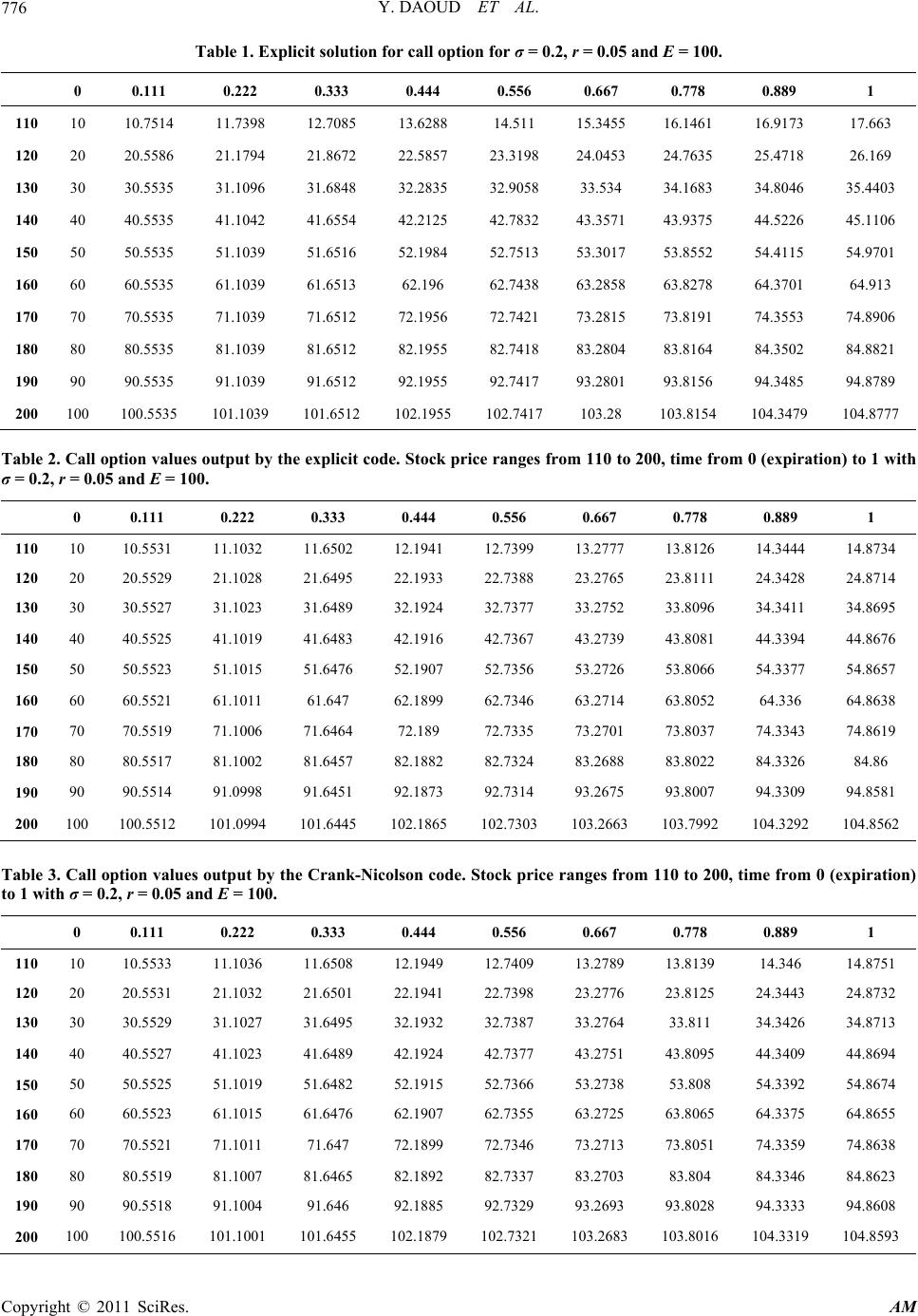

Y. DAOUD ET AL. 776
Table 1. Explicit solution for call option for σ = 0.2, r = 0.05 and E = 100.
0 0.111 0.222 0.333 0.444 0.556 0.667 0.778 0.889 1
110 10 10.7514 11.7398 12.7085 13.6288 14.511 15.3455 16.1461 16.9173 17.663
120 20 20.5586 21.1794 21.8672 22.5857 23.3198 24.0453 24.7635 25.4718 26.169
130 30 30.5535 31.1096 31.6848 32.2835 32.9058 33.534 34.1683 34.8046 35.4403
140 40 40.5535 41.1042 41.6554 42.2125 42.7832 43.3571 43.9375 44.5226 45.1106
150 50 50.5535 51.1039 51.6516 52.1984 52.7513 53.3017 53.8552 54.4115 54.9701
160 60 60.5535 61.1039 61.6513 62.196 62.7438 63.2858 63.8278 64.3701 64.913
170 70 70.5535 71.1039 71.6512 72.1956 72.7421 73.2815 73.8191 74.3553 74.8906
180 80 80.5535 81.1039 81.6512 82.1955 82.7418 83.2804 83.8164 84.3502 84.8821
190 90 90.5535 91.1039 91.6512 92.1955 92.7417 93.2801 93.8156 94.3485 94.8789
200 100 100.5535 101.1039 101.6512 102.1955 102.7417 103.28 103.8154 104.3479 104.8777
Table 2. Call option values output by the explicit code. Stock price ranges from 110 to 200, time from 0 (expiration) to 1 with
σ = 0.2, r = 0.05 and E = 100.
0 0.111 0.222 0.333 0.444 0.556 0.667 0.778 0.889 1
110 10 10.5531 11.1032 11.6502 12.1941 12.7399 13.2777 13.8126 14.3444 14.8734
120 20 20.5529 21.1028 21.6495 22.1933 22.7388 23.2765 23.8111 24.3428 24.8714
130 30 30.5527 31.1023 31.6489 32.1924 32.7377 33.2752 33.8096 34.3411 34.8695
140 40 40.5525 41.1019 41.6483 42.1916 42.7367 43.2739 43.8081 44.3394 44.8676
150 50 50.5523 51.1015 51.6476 52.1907 52.7356 53.2726 53.8066 54.3377 54.8657
160 60 60.5521 61.1011 61.647 62.1899 62.7346 63.2714 63.8052 64.336 64.8638
170 70 70.5519 71.1006 71.6464 72.189 72.7335 73.2701 73.8037 74.3343 74.8619
180 80 80.5517 81.1002 81.6457 82.1882 82.7324 83.2688 83.8022 84.3326 84.86
190 90 90.5514 91.0998 91.6451 92.1873 92.7314 93.2675 93.8007 94.3309 94.8581
200 100 100.5512 101.0994 101.6445 102.1865 102.7303 103.2663 103.7992 104.3292 104.8562
Table 3. Call option values output by the Crank-Nicolson code. Stock price ranges from 110 to 200, time from 0 (expiration)
to 1 with σ = 0.2, r = 0.05 and E = 100.
0 0.111 0.222 0.333 0.444 0.556 0.667 0.778 0.889 1
110 10 10.5533 11.1036 11.6508 12.1949 12.7409 13.2789 13.8139 14.346 14.8751
120 20 20.5531 21.1032 21.6501 22.1941 22.7398 23.2776 23.8125 24.3443 24.8732
130 30 30.5529 31.1027 31.6495 32.1932 32.7387 33.2764 33.811 34.3426 34.8713
140 40 40.5527 41.1023 41.6489 42.1924 42.7377 43.2751 43.8095 44.3409 44.8694
150 50 50.5525 51.1019 51.6482 52.1915 52.7366 53.2738 53.808 54.3392 54.8674
160 60 60.5523 61.1015 61.6476 62.1907 62.7355 63.2725 63.8065 64.3375 64.8655
170 70 70.5521 71.1011 71.647 72.1899 72.7346 73.2713 73.8051 74.3359 74.8638
180 80 80.5519 81.1007 81.6465 82.1892 82.7337 83.2703 83.804 84.3346 84.8623
190 90 90.5518 91.1004 91.646 92.1885 92.7329 93.2693 93.8028 94.3333 94.8608
200 100 100.5516 101.1001 101.6455 102.1879 102.7321 103.2683 103.8016 104.3319 104.8593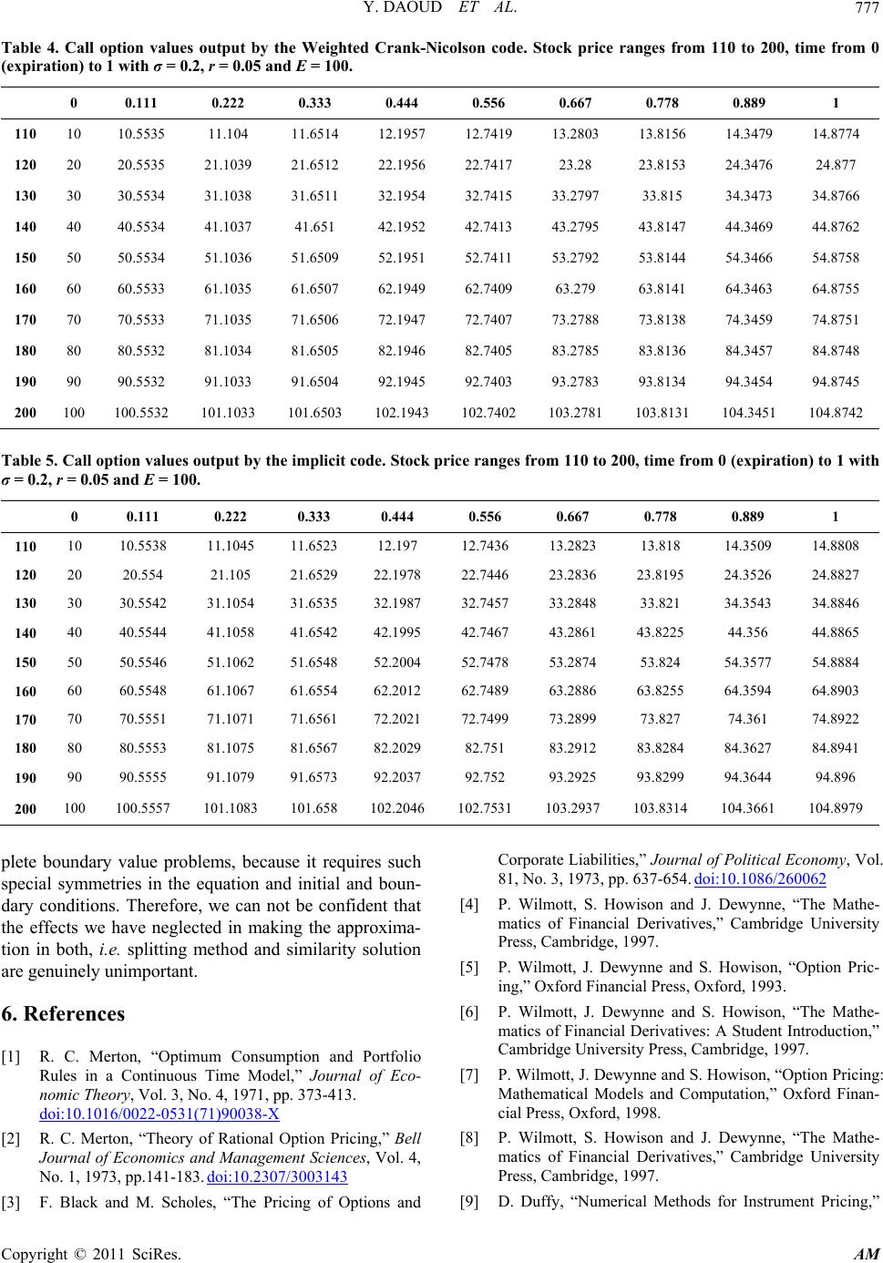

Y. DAOUD ET AL.777
Table 4. Call option values output by the Weighted Crank-Nicolson code. Stock price ranges from 110 to 200, time from 0
(expiration) to 1 with σ = 0.2, r = 0.05 and E = 100.
0 0.111 0.222 0.333 0.444 0.556 0.667 0.778 0.889 1
110 10 10.5535 11.104 11.6514 12.1957 12.7419 13.2803 13.8156 14.3479 14.8774
120 20 20.5535 21.1039 21.6512 22.1956 22.7417 23.28 23.8153 24.3476 24.877
130 30 30.5534 31.1038 31.6511 32.1954 32.7415 33.2797 33.815 34.3473 34.8766
140 40 40.5534 41.1037 41.651 42.1952 42.7413 43.2795 43.8147 44.3469 44.8762
150 50 50.5534 51.1036 51.6509 52.1951 52.7411 53.2792 53.8144 54.3466 54.8758
160 60 60.5533 61.1035 61.6507 62.1949 62.7409 63.279 63.8141 64.3463 64.8755
170 70 70.5533 71.1035 71.6506 72.1947 72.7407 73.2788 73.8138 74.3459 74.8751
180 80 80.5532 81.1034 81.6505 82.1946 82.7405 83.2785 83.8136 84.3457 84.8748
190 90 90.5532 91.1033 91.6504 92.1945 92.7403 93.2783 93.8134 94.3454 94.8745
200 100 100.5532 101.1033 101.6503 102.1943 102.7402 103.2781 103.8131 104.3451 104.8742
Table 5. Call option values output by the implicit code. Stock price ranges from 110 to 200, time from 0 (expiration) to 1 with
σ = 0.2, r = 0.05 and E = 100.
0 0.111 0.222 0.333 0.444 0.556 0.667 0.778 0.889 1
110 10 10.5538 11.1045 11.6523 12.197 12.7436 13.2823 13.818 14.3509 14.8808
120 20 20.554 21.105 21.6529 22.1978 22.7446 23.2836 23.8195 24.3526 24.8827
130 30 30.5542 31.1054 31.6535 32.1987 32.7457 33.2848 33.821 34.3543 34.8846
140 40 40.5544 41.1058 41.6542 42.1995 42.7467 43.2861 43.8225 44.356 44.8865
150 50 50.5546 51.1062 51.6548 52.2004 52.7478 53.2874 53.824 54.3577 54.8884
160 60 60.5548 61.1067 61.6554 62.2012 62.7489 63.2886 63.8255 64.3594 64.8903
170 70 70.5551 71.1071 71.6561 72.2021 72.7499 73.2899 73.827 74.361 74.8922
180 80 80.5553 81.1075 81.6567 82.2029 82.751 83.2912 83.8284 84.3627 84.8941
190 90 90.5555 91.1079 91.6573 92.2037 92.752 93.2925 93.8299 94.3644 94.896
200 100 100.5557 101.1083 101.658 102.2046 102.7531 103.2937 103.8314 104.3661 104.8979
plete boundary value problems, because it requires such
special symmetries in the equation and initial and boun-
dary conditions. Therefore, we can not be confident that
the effects we have neglected in making the approxima-
tion in both, i.e. splitting method and similarity solution
are genuinely unimportant.
6. References
[1] R. C. Merton, “Optimum Consumption and Portfolio
Rules in a Continuous Time Model,” Journal of Eco-
nomic Theory, Vol. 3, No. 4, 1971, pp. 373-413.
doi:10.1016/0022-0531(71)90038-X
[2] R. C. Merton, “Theory of Rational Option Pricing,” Bell
Journal of Economics and Management Sciences, Vol. 4,
No. 1, 1973, pp.141-183. doi:10.2307/3003143
[3] F. Black and M. Scholes, “The Pricing of Options and
Corporate Liabilities,” Journal of Political Economy, Vol.
81, No. 3, 1973, pp. 637-654. doi:10.1086/260062
[4] P. Wilmott, S. Howison and J. Dewynne, “The Mathe-
matics of Financial Derivatives,” Cambridge University
Press, Cambridge, 1997.
[5] P. Wilmott, J. Dewynne and S. Howison, “Option Pric-
ing,” Oxford Financial Press, Oxford, 1993.
[6] P. Wilmott, J. Dewynne and S. Howison, “The Mathe-
matics of Financial Derivatives: A Student Introduction,”
Cambridge University Press, Cambridge, 1997.
[7] P. Wilmott, J. Dewynne and S. Howison, “Option Pricing:
Mathematical Models and Computation,” Oxford Finan-
cial Press, Oxford, 1998.
[8] P. Wilmott, S. Howison and J. Dewynne, “The Mathe-
matics of Financial Derivatives,” Cambridge University
Press, Cambridge, 1997.
[9] D. Duffy, “Numerical Methods for Instrument Pricing,”

Y. DAOUD ET AL. 778
John Wiley & Sons, Chichester, 2004.
[10] D. J. Duffy, “Financial Instrument Pricing in C++,” John
Wiley & Sons, Chichester, 2004.
[11] J. Geiser, “Decomposition Methods for Differential
Equations Theory and Applications,” Chapman Hall/CRC
Press, London, 2009. doi:10.1201/9781439810972
[12] I. Farago and J. Geiser, “Iterative Operator Splitting
Methods for Linear Problems,” International Journal of
Computational Science and Engineering, Vol. 3, No. 4,
2007, pp. 255-263.
[13] P. Csomo’s, I. Farago and A. Havasi, “Weighted Sequen-
tial Splitting and Their Analysis,” Computers & Mathe-
matics with Applications, Vol. 50, 2005, pp. 1017-1031.
doi:10.1016/j.camwa.2005.08.004
[14] J. Geiser, “Linear and Quasi-Linear Iterative Splitting
Methods: Theory and Applications,” International Mathe-
matical Forum, Vol. 2, No. 49, 2007, pp. 2391-2416.