 Applied Mathematics, 2011, 2, 757-763 doi:10.4236/am.2011.26101 Published Online June 2011 (http://www.SciRP.org/journal/am) Copyright © 2011 SciRes. AM Conditionally Suboptimal Filtering in Nonlinear Stochastic Differential System* Tongjun He, Zhengping Shi College of Mathem at i cs an d C om put er Science, Fuzhou University, Fuzh ou, China E-mail: hetongjun@fzu.edu.cn, shizp@fzu.edu.cn Received January 25, 2011; revised April 27, 2011; accepted April 30, 2011 Abstract This paper presents a novel conditionally suboptimal filtering algorithm on estimation problems that arise in discrete nonlinear time-varying stochastic difference systems. The suboptimal state estimate is formed by summing of conditionally nonlinear filtering estimates that their weights depend only on time instants, in contrast to conditionally optimal filtering, the proposed conditionally suboptimal filtering allows parallel processing of information and reduce online computational requirements in some nonlinear stochastic dif- ference system. High accuracy and efficiency of the conditionally suboptimal nonlinear filtering are demon- strated on a numerical example. Keywords: Suboptimal Estimate, Conditionally Filter, Nonlinear Stochastic System 1. Introduction Some simple Kalman-Bucy filters [1-4] lead to some conditionally optimal filtering [5-7]. This main idea is that the absolute unconditional optimality is rejected and in a class of admissible estimates with some nonlinear stochastic differential equations or nonlinear stochastic difference equations that can be solved online while re- ceiving the results of the measurements, the optimal es- timate is found. In this paper we are interesting in con- stituting a novel conditionally filtering algorithm ad- dressing estimation problems that suboptimal arise in discrete nonlinear time-varying stochastic difference systems with different types of measurements [8-10]. By a weighted sum of local conditionally nonlinear stochas- tic filtering estimates, the suboptimal estimate of state of this conditionally nonlinear stochastic filtering is given, thus due to its inherent parallel structure, it can be im- plemented on a set of parallel processors. The aim of this paper is to give an alternative conditionally suboptimal filtering for that kind of discrete time nonlinear stochas- tic difference systems. As same as the conditionally op- timal filtering, the conditionally suboptimal filtering represents the state estimate as a weighted sum of local conditionally filtering estimates associated with the weights depending only on time instants and being inde- pendent of current measurements. 2. Problem Statement for Nonlinear Stochastic Difference Systems In [6], consider a nonlinear discrete stochastic system whose state vector is determined by a nonlin- ear stochastic difference system n lRX 100 1 n lllll rllr r aac c XX X l V. (1) Suppose that the observation vector l is composed of differential types of observation sub-vectors, i.e., Y N T ,, iN ll l YYY , (2) where 1 i li Y is determined by the stochastic system, 00 1 n i ii llll lrllr r bbd d YX X ii l V, (3) in (1) and (3), lr is the rth component of the vector l , is discrete time, are the matrices, 00ll are the constant vectors of the respec- tive dimension, l 00 ,,, ,, iii ll rl llrl acc bdd i b,a l V is a sequence of independent ran- dom variables with known distribution. We shall also assume that 1) The state sequence of random variables l and the measurement noise sequence of random variables l V are independent of each other, so that *The authors were partially supported by NSFC(11001054) and the Found of the Ministry of Education of Fujian Province: JA090022.  T. J. HE ET AL. 758 0, . T ijiji j EVVEX VEXEV 2) The random variables is a sequence of Gaus- sian white noise with zero mean and covariance matrix l V T ll l EVVG I . (4) Usually, for a fixed , the conditionally optimal filter is to find an estimate 1iiN ˆi l of the random state variable l at each discrete time by the meas- urements of the previous random variables l 11 ,, ii l YY , here, the class of admissible estimates are defined by the difference equation 111 1 ˆδ, iiiiii i lllll XAUYA 1 i l (5) with a given sequence of the vector structural functions and all possible values of the matrices of coefficients and the coefficients vectors 1, i luy 1 δi l 1 i l . The class of admissible filtering is determined by the given sequence of the structural functions 1. Cer- tainly, such an estimate i l ,uy ˆi l is required to minimize the mean square error in some sense 2 ˆi ll EX X (6) at any discrete time l. This problem arises from the multi-criteria equation, δ, ii ll can be optimal. Our problem is to find a suboptimal estimate * ˆl at any discrete time by using different types of esti- mates l ,, N 1 ˆˆ l XXl such that 2 * ˆll EX X (7) is minimal in some sense. 3. Construction of Conditionally Suboptimal Nonlinear Filter 3.1. Conditionally Nonlinear Filter For , we firstly choose a sequence of struc- tural functions 1iiN ˆ ,T iii ii TT lll ll UY XY , let I, and substitute into (5) we can derive that 11 2 ˆˆˆ δδ iiiii lllll XXY i l , (8) where l , 12 δδδ iii ll ˆ1, 2,, i ll Ui N, this is a class of admissible filters. The conditionally optimal nonlinear filtering is consist of (1), (3) and (8), and it is denoted by . Applying conditionally optimal nonlinear filter theory [5] we obtain the following results for this conditionally optimal nonlinear filtering : If 22 1, , iii i T lll l bRbH iN is inverse, then 1 212 δi iiiiiii TT llll llll l aR bHbR bH22 (9) 12 δδ ii llll ab i ii l , (10) 010 δ i lll ab , (11) for any 1, 2,,ii N n , where TT 11 0000 1 T ,1 ll lllrllrlrl ll r n lrlslrsrll sl rs Hc GcmcGccGc mmk cGc T T i T , (12) TT 12 0000 1 T ,1 n ii i lllllrll rlrlll r ni lrlslrsrll sl rs HcGdmcGdcGd mmk cGd , (13) TT 22 0000 1 T ,1 n iiiii ii lllllrll rlrlll r nii lrlslrsrll sl rs HdGdmdGddGd mmkdGd , (14) l G lr is the covariance matrix of the random vector l, V m 1, 2,,r EX n , are the components of the vector ll m , ,1,,s n lrs kr are the elements of the covariance matrix lxl K of the random vector l . Substitute (10) and (11) into (8) we obtain a sequence of conditionally optimal filtering equations 102 ˆˆ ˆ δ ii iiii lllllllll0 i aXaYb Xb . (15) This is the usual Kalman filtering equation, but in more general problem, Equations (1) and (3) are nonlin- ear, the matrix coefficient 2 is determined by Formu- las (9) and (12)-(14) that are different from the corre- sponding formula of Kalman linear filtering theory. δl Let , ll mEX T lllll EX mX m , , iii T lll REXX where l ˆ ii ll XX is the error of filtering. To give out the solution of this problem, it is necessary to indi- cate how the expectation and the covariance matrix l m l of the random vector l and the covariance matrix l of the error of filtering l R can be found at each step. For this purpose, we can deduce from (1) and (15) the stochastic difference equation for the error of filter- ing l 12 20 02 1 δ δδ iiii lllll n ii ii llll rlrllrl r XabX dc dcXV (16) for any 1, ,ii N. Taking into account that l , Copyright © 2011 SciRes. AM  T. J. HE ET AL.759 l are independent of land the unbiaseness of esti- mate l V ˆˆ ii ll EX EX, we can deduce from (1) and (16) that the difference equations for , l ml , , l R 1ll 1 0l ma l ma ll , (17) 11 T lll aKa i ll b H 1 2 δ ii llll RaRa 1, ,ii N m , (18) ii TT ll Ra 12l H11 T l H i, (19) for any . Remark 3.1 l, l , l, 2 are determined by the Equations (17)-(19) and the Equations (9), (17), (18) are linear difference equations, so l, l Rδl m are deter- mined successively. However, it follows from the for- mula (9) that 2 depends on l, therefore, Equation (19) is nonlinear difference equation with respect to . δlR l R 3.2. Conditionally Suboptimal Nonlinear Filter Next, we start with the suboptimal estimate of condition- ally nonlinear filtering , it follows from (15) and (19) that the conditionally nonlinear filtering has filtering estimates ll l N ˆ , i 2 ˆˆ ,, N XX * at each step. Then the suboptimal estimate ˆl for the conditionally non- linear filtering I is constructed from these estimates 12 ˆˆ ˆ ,,, ll l XX * by the following equations 1 ˆˆ ii ll N ii ll i XpX pp 1 0, N i l I , (20) where is an unit matrix, 12 ,, , lll are posi- tive semi-definite matrices and weighted coefficients that are determined by the following mean square criterion, pp p * 2 * 1 ˆ min l N ll l i XEX XEX 2 ˆˆ ii l p X min i l pl ˆl . (21) Remark 3.2 The suboptimal estimate * is unbi- ased. Since each estimate ˆi l ,1, 2, i i l EX l X N l ,N l EX l is unbi- ased, , using (20), we can obtain 1, i ll EXEX i 2, l * 11 ˆˆ NN ii ll ii EXp EXp . (22) 3.3. The Accuracy of Conditionally Suboptimal Nonlinear Filter Now, we derive the equation for the actual variance ma- trix * ˆ , , T ll l REXXX X (23) where l is the state vector (1), * l ˆ is the suboptimal filtering estimate (20), and 1 ˆ , , Niiii lllll il pX XXX 0 n (24) substitute (24) into (23) we can derive that 1 ,1, , N Niiiiij j TT lllllll iiji j RpRp pRp (25) where is determined by Equation (19), is determined by the following formula i l R ij l R 1 220 00 11 ,1 δδ ; ,1,,, ijij T lll T iiijj jij lllllll lll nn ij ij TT lrll rllr rlll rr nij T lrs rll sl rs REXX abRab QGQ mQ GQmQGQ kQGQi jijN (26) where 0200 2 δ, δ 1,, iii iii llllrllrlrl QdcQdci The question is that there is a sequence of positive semi-definite matrices 12 ,,, lll pp p 12 such that (21) has a minimal value. Here, we point out that the equa- tions of the optimal coefficients ,,, ll pp l p have the following form, 2 1 1 22 1 0, NT jkj Nj lll kj l T NkNN ll l Niik iN ll i Nk N N ll l tr RpRR p pR R pR R pR R (27) for any 1, ,1kN , 1N ll ppI . (28) The proof of these equations is given in the Appendix. Then the actual variance matrix of the filtering error l and the actual mean square error can be calcu- lated by using the formula (25) and Equations (19), (26), (27). Thus the Equations (9), (12), (13), (14), (19), (26), and (27) completely define the new suboptimal linear filter for estimate R l tr R * ˆl of the state vector l . Note that the Equations (9), (12), (13), (14), (19), and (26) are separated for any 1,, Nii. Therefore, they can be solved in parallel. 4. Example Consider the problem of recursive estimate of an un- known scalar parameter [4]. To estimate the value of the Copyright © 2011 SciRes. AM  T. J. HE ET AL. 760 unknown parameter from two types of observations corrupted by additive white noises, the observation mod- els of the stochastic system are given by 1001lllllll l aXaccXV , (29) 11111 001llll lll YbXbddX l V l V , (30) 22222 001lllllll YbXbddX, (31) where l , l, l, and are in- dependent Gaussian noises, 1 2 YYR 0,1 l VN 000 ˆ, NX P . The op- timal filtering estimates 1 ˆl , 2 ˆl based on observa- tion system (30), (31) is determined by the structural functions, respectively, 11111 11 2 ˆˆ δδ lllll XXY 1 l , (32) 22222 11 2 ˆˆ δδ lllll XXY 2 l . (33) Then such this problem is a conditionally nonlinear filtering estimation problem, and applying conditionally nonlinear filtering theory, it follows from (9), (10), (11), (12), (13), and (14) that 1lll mama 0l 11 l , (34) 1llll aKa H , (35) where 2 11 000 11 1 2 llllllllll lll cGcmcGcmK cGc , (36) and 1 11111111 212 δllll llll l aRbHbRbH 22 (37) 11 111 1112 δ lllll lllll RaRa HbRa H 1 12 1 1 l 1 22 l 2 2 , (38) 11 12 δδ llll ab , (39) 11 020 δ lll ab , (40) where 111 120 11 0 1 2 00 11 , llllllll lllllll l HmcGdcGd cGdmK cGd (41) 11111 220 110 11 11 2 00 11 , llllllll llllll ll HmdGddGd dGdm KdGd (42) and 1 22222222 212 δ, lllllllll aRbHbRbH (43) 2222 22 1 21211 δ, lllllllll RbRa HaRa H (44) 22 12 δδ llll ab , (45) 22 020 δ lll ab , (46) where 222 120 11 0 22 2 00 11 , llllllll lllllll l HmcGdcGd cGdmK cGd (47) 22222 220 110 22 22 2 00 11 . llllllll llllllll HmdGddGd dGdm KdGd (48) Next, we will compute conditionally suboptimal non- linear filtering with two different types of observations and the error variance matrix . Firstly, we need com- pute covariance l R 121 1122212 12 200 12 1212 00 1011 δδ , llllllll lll llll llllllll RabRabQGQ mQ GQmQ GQKQ GQ (49) 2122211 121 12 20 21 2121 00 1011 δδ , llllllllll llllll llllll RabRabQGQ mQ GQmQ GQKQ GQ 0l 0l c (50) where 1112 22 02000 20 δ, δ lllll ll QdcQ d , 1112 22 12111 21 δ, δ lllll ll QdcQ d 1l c Secondly, we will find two weighted coefficients i l p 1, 2i such that the error variance l is minimal. It follows from Equation (27) at that R 2N 11122 212 12 0 , llll ll ll pR RpRR ppI (51) moreover, we can derive from (51) that 221 1 1 2 1221 ll l ll ll RR pRRR R , (52) 112 2 1 2 1221 ll l ll ll RR pRRR R , (53) it follows from (20) that the suboptimal estimate 112 2 * ˆˆ ˆ lllll pX pX, (54) and according to (25) the suboptimal estimation variance of error has the form: l R 1112 2 2 112 22 211 , llll lll llll ll RpRppRp pR ppRp (55) where , are determined by Equations (38), (44), respectively; and , are determined by Equations (49), (50), respectively; , are de- 1 l R 2 l R 12 l R 21 l R 1 l p 2 l p Copyright © 2011 SciRes. AM 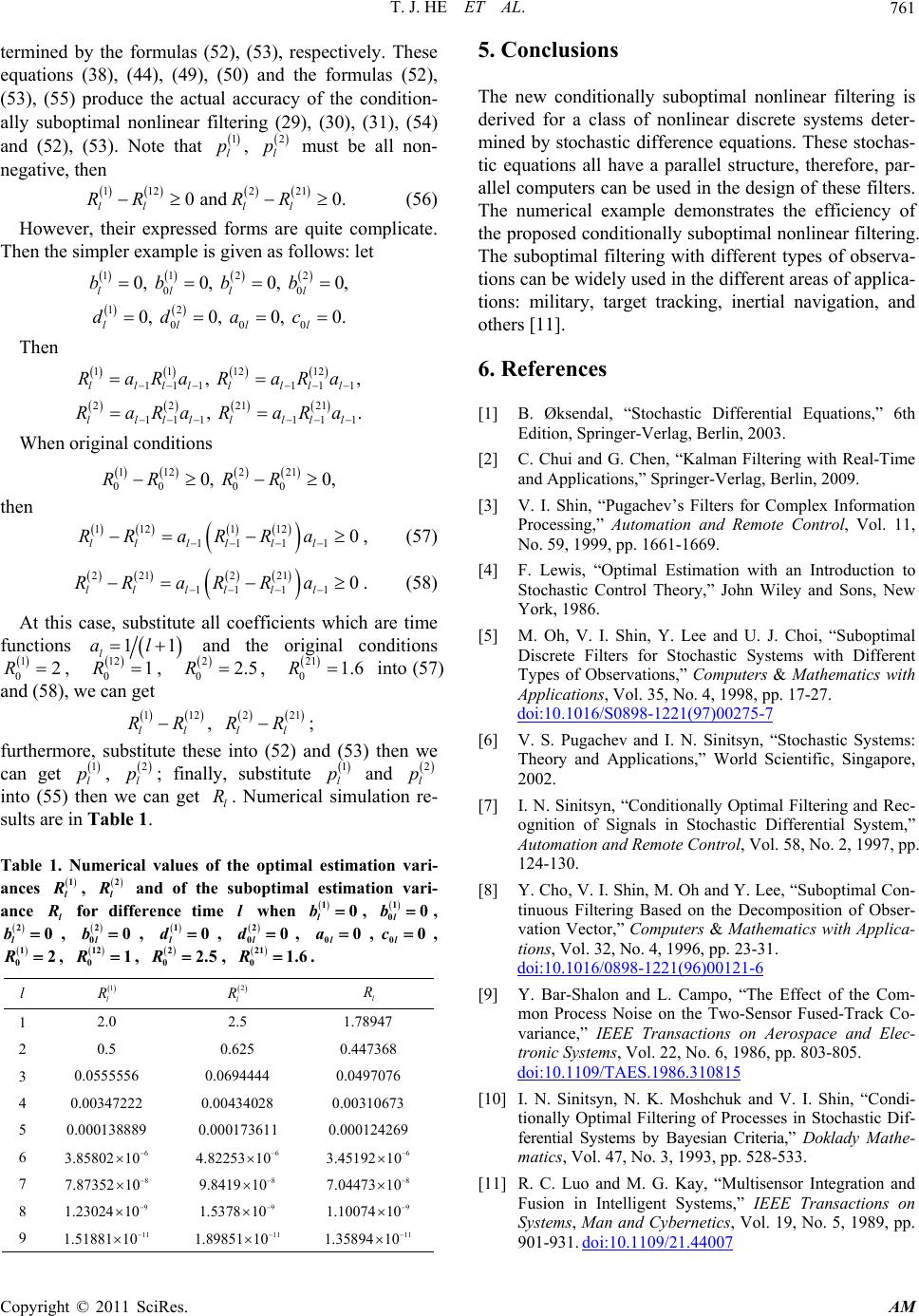 T. J. HE ET AL. Copyright © 2011 SciRes. AM 761 5. Conclusions termined by the formulas (52), (53), respectively. These equations (38), (44), (49), (50) and the formulas (52), (53), (55) produce the actual accuracy of the condition- ally suboptimal nonlinear filtering (29), (30), (31), (54) and (52), (53). Note that , must be all non- negative, then 1 l p and 0, 00 , 12 1l R 21 1l R 0, R 11ll R 11ll R 2 l p 2 l R 2 00l 0, l a , ,a , . l a 2 0 0,R 1 l R 2 l R The new conditionally suboptimal nonlinear filtering is derived for a class of nonlinear discrete systems deter- mined by stochastic difference equations. These stochas- tic equations all have a parallel structure, therefore, par- allel computers can be used in the design of these filters. The numerical example demonstrates the efficiency of the proposed conditionally suboptimal nonlinear filtering. The suboptimal filtering with different types of observa- tions can be widely used in the different areas of applica- tions: military, target tracking, inertial navigation, and others [11]. 11221 0 0. ll l RR R (56) However, their expressed forms are quite complicate. Then the simpler example is given as follows: let 11 2 0, 0, 0, ll l bbbb 12 0 0, 0 0. ll l dd c Then 6. References 1 112 1111 1lllllll RaRa Ra 2 221 1111 1lll lll RaRa Ra [1] B. Øksendal, “Stochastic Differential Equations,” 6th Edition, Springer-Verlag, Berlin, 2003. When original conditions [2] C. Chui and G. Chen, “Kalman Filtering with Real-Time and Applications,” Springer-Verlag, Berlin, 2009. 11221 00 0 RR [3] V. I. Shin, “Pugachev’s Filters for Complex Information Processing,” Automation and Remote Control, Vol. 11, No. 59, 1999, pp. 1661-1669. then 11212 1 1 0 ll l RR aa , (57) 221 21 1 1 0 ll l RR aa . (58) [4] F. Lewis, “Optimal Estimation with an Introduction to Stochastic Control Theory,” John Wiley and Sons, New York, 1986. At this case, substitute all coefficients which are time functions 11 l al and the original conditions , , , into (57) and (58), we can get 1 02R 12 01R [5] M. Oh, V. I. Shin, Y. Lee and U. J. Choi, “Suboptimal Discrete Filters for Stochastic Systems with Different Types of Observations,” Computers & Mathematics with Applications, Vol. 35, No. 4, 1998, pp. 17-27. doi:10.1016/S0898-1221(97)00275-7 2. 2 R l R 2 0 R5R 22 ll R 21 01.6 11 ll RR, ; 1 [6] V. S. Pugachev and I. N. Sinitsyn, “Stochastic Systems: Theory and Applications,” World Scientific, Singapore, 2002. furthermore, substitute these into (52) and (53) then we can get , ; finally, substitute and into (55) then we can get . Numerical simulation re- sults are in Table 1. 1 l p 2 l p 1 l p 2 l p [7] I. N. Sinitsyn, “Conditionally Optimal Filtering and Rec- ognition of Signals in Stochastic Differential System,” Automation and Remote Control, Vol. 58, No. 2, 1997, pp. 124-130. Table 1. Numerical values of the optimal estimation vari- ances 1 l , 2 l and of the suboptimal estimation vari- ance l for difference time when , [8] Y. Cho, V. I. Shin, M. Oh and Y. Lee, “Suboptimal Con- tinuous Filtering Based on the Decomposition of Obser- vation Vector,” Computers & Mathematics with Applica- tions, Vol. 32, No. 4, 1996, pp. 23-31. doi:10.1016/0898-1221(96)00121-6 l 10 l b 1 00 l b , , , , , , 2 l b0b 2 00 l 10 l d 20 l 0 d00 l a00 l c , , , , . 1 0 R2R 12 01 2 0 R2.5 R 21 1.6 0 l 1 l 2 l l [9] Y. Bar-Shalon and L. Campo, “The Effect of the Com- mon Process Noise on the Two-Sensor Fused-Track Co- variance,” IEEE Transactions on Aerospace and Elec- tronic Systems, Vol. 22, No. 6, 1986, pp. 803-805. doi:10.1109/TAES.1986.310815 1 2.0 2.5 1.78947 2 0.5 0.62 0.0694 0.004340 000173 4.82253 5 0.447368 3 0.0555556 444 28 611 6 10 0.0497076 4 0.00347222 0.00310673 5 0.000138889 0. 0.000124269 6 6 3.85802 10 6 3.45192 10 7 8 7.87352 10 [10] I. N. Sinitsyn, N. K. Moshchuk and V. I. Shin, “Condi- tionally Optimal Filtering of Processes in Stochastic Dif- ferential Systems by Bayesian Criteria,” Doklady Mathe- matics, Vol. 47, No. 3, 1993, pp. 528-533. [11] R. C. Luo and M. G. Kay, “Multisensor Integration and Fusion in Intelligent Systems,” IEEE Transactions on Systems, Man and Cybernetics, Vol. 19, No. 5, 1989, pp. 901-931. doi:10.1109/21.44007 8 10 9.8419 8 7.0447310 8 9 1.23024 10 1.53789 10 9 1.10074 10 9 11 1.51881 10 1.89851 11 10 11 1.3589410  T. J. HE ET AL. 762 00 c Appendix Derivation of Formula (26). It follows from (16) that 111 2112 2002 00 20 02 1 2 1 δδ δδ δδ δ ijijT lll T iiijj j T llllllll T iij j T llllll ll T n iij j T llllllrlrllr r ii lrlrl r REXX abEXXab dcEVV dc dcEVVdcX dc 2 1 22 1 δ δδ, nT lrl l T njj T lrlrlrl r nT iij j T lrlrllrlll ll r XEVV Xdc dcXEVV dc (56) set 0 , 020 δ iii lll Qd l c 2 iii rllrlrl Qd , then it fol- lows from (56) that 122 0 00 11 1 δδ ;,1,,. T ijiiiji iijT lllllllll ll nn ij ij TT lrll rllr rlll rr nij T lrs rll sl r RabRaabQGQ mQGQmQ GQ kQGQi jijN 0 l l (57) Derivation of Equation (27). We seek the optimal ma- trices minimizing the mean square error, i.e., 1, , i l pi N 1,1, NN iiiiij j TT llllll iijij trRtr pRptr pRp (58) 1, 0. Nii ll ipIp (59) Next, we use the following formulae , , TT T tr ABAABAB A trABtr BAB AA (60) to differentiate the function with respect to , we can derive that for any , l tr R k l p 1, ,1kN k 1 ,1, , Niii T llll kk i ll Niijj T lll kiji j l tr RtrpRp pp tr pRp p substitute (59) into the following equation, we can derive that for any , k 1 11 22 2 22, Niii T lll ki l kkN ll l NN lll l kk NN llll tr pRp p pRR ppp p pRp R (62) ,1, 1 ,1, 1 1 1 1 , Niijj T ll l kijij l Niij j T ll l kiji j l NNNj j T ll l kj l NiiNN T ll l ki l tr pRp p tr pRp p tr pRp p tr pRp p (63) 1 ,1, 11 1, 1, . Niij j T ll l kijij l NN kji ik T ll ll jjk iik tr pRp p pR pR (64) Substitute (59) into the following equations, we can derive that 1 1 11() 1 1 11 1, 1, ( , NiiNN T ll l ki l NT N iiN j ll l j ki l kNk kNk kN TTT lllll NN jkN iiN TT ll ll jjk iik tr pRp p tr pRIp p RpRpR pR pR (65) (61) 1 1 11 1 1 11 1, 1, ( NNNj j T ll l kj l NNjNjj T lll j ki l T NkkkNk Nk lll ll NN T jNj iNk ll ll jjk iik tr pRp p tr IpRp p RpRpR pR pR (66) for any k 1, ,1kN . Substitute (62)-(66) into 61), we can derive that ( Copyright © 2011 SciRes. AM  T. J. HE ET AL. Copyright © 2011 SciRes. AM 763 1 1, 1 1, 11 11 2 NTT jkj Njkkk Nk lllllll kjjk l Niik iNkkk kN llll ll iik NN TTT jkNikNkNNk N llllll ll ji tr RpRRpRR p pR RpRR pRpRRR pR 1 1 1 1 , N NT T jkj NjNkN N llllll j NiikiNNNk N llll ll i pR RpRR pRRp RR (67) let the result be zero, we get (27).
|