 Applied Mathematics, 2011, 2, 739-749 doi:10.4236/am.2011.26098 Published Online June 2011 (http://www.SciRP.org/journal/am) Copyright © 2011 SciRes. AM Septic B-Spline Collocation Method for the Numerica l Solution of the Modified Equal Width Wave Equation Turabi Geyikli, Seydi Battal Gazi Karakoc Department of Mathematics, Faculty of Education, Inonu University, Malatya, Turkey E-mail: tgeyikli@inonu.edu.tr, sbgk44@mynet.com Received March 25, 2011; revised April 20, 2011; accepted April 23, 2011 Abstract Numerical solutions of the modified equal width wave equation are obtained by using collocation method with septic B-spline finite elements with three different linearization techniques. The motion of a single soli- tary wave, interaction of two solitary waves and birth of solitons are studied using the proposed method. Accuracy of the method is discussed by computing the numerical conserved laws error norms L2 and L∞. The numerical results show that the present method is a remarkably successful numerical technique for solving the MEW equation. A linear stability analysis shows that this numerical scheme, based on a Crank Nicolson approximation in time, is unconditionally stable. Keywords: Finite Element, Septic B-Spline, Collocation, Soliton, Solitary Waves 1. Introduction This study is concerned with the numerical solution, us- ing septic B-spline functions in collocation method, of the modified equal width wave (MEW) equation, which was introduced by Morrison et al. [1] as a model equa- tion to describe the nonlinear dispersive waves. Few analytical solutions of the MEW equation are known. Thus numerical solutions of the MEW equation can be important and comparison between analytic solution can be made. Many methods have been proposed to solve the EW and MEW equation. Gardner and Gardner solved the EW equation with the Galerkin’s method using cubic B-splines as a trial and test function [2,3] and a Pet- rov-Galerkin method using quadratic B-spline element [4]. Zaki considered the solitary wave interactions for the MEW equation by Petrov-Galerkin method using quintic B-spline finite elements [5] and obtained the numerical solution of the EW equation by using least-squares method [6]. Wazwaz investigated the MEW equation and two of its variants by the tanh and the sine-cosine meth- ods [7]. Esen applied a lumped Galerkin method based on quadratic B-spline finite element has been used for solving the EW and MEW equation [8,9]. Saka proposed algorithms for the numerical solution of the MEW equa- tion using quintic B-spline collocation method [10]. A solution based on a collocation method incorporated cu- bic B-splines is investigated by Dağ and Saka [11]. Variational iteration method is introduced to solve the MEW equation by Junfeng Lu [12]. Hamdi et al. [13] derived exact solitary wave solutions of the generalized EW equation using Maple software. D. J. Evans and K. R. Raslan [14] studied the generalized EW equation by using collocation method based on quadratic B-splines to obtain the numerical solutions of a single solitary waves, and the birth of solitons. The modified equal width wave equation which is as a model for non-linear dispersive waves, considered here has the normalized form [1] 2 3 tx xxt UUU U 0 (1) with the physical boundary conditions as , where is time and 0U x t is the space coordi- nate, is a positive parameter. For this study bound- ary conditions are chosen ,0, ,0, ,0, ,0, ,0, ,0 xx xxx xxx Uat Ubt Uat Ubt Uat Ubt , (2) and the initial condition as ,0, Uxfxaxb where x is a localized disturbance inside the con- sidered interval.  T. GEYIKLI ET AL. 740 2. Septic B-Spline Collocation Method The interval ,ab is partitioned into uniformly sized finite elements by the knots i such that 01 N ax xxb and . The septic 1ii hx x B-splines i , (i= −3(1) N + 3), at the knots i are defined over the interval ,ab as [15], 7 443 77 43 3 77 7 43 22 777 7 43211 777 7 74321 ,, 8, , 828, , 82856,, 1( )8()28( )56(),,, iii ii i ii ii ii i ii iii i iii i xxx xx xxxxx x x xxxxxxx xx xxxxxxxxxxx xxx xxxxxxxxx h x 777 43 21 77 43 2 7 434 828, , 8, , ,, 0o ii i ii i iii xxx xxxxx xx xxxxx x xxxx 2 1 1 , , , , i i i 2 3 , , , therwise. i i (3) The set of splines, 32 3 ,,, N x x forms a basis for functions defined over ,ab . The numerical solution to takes the form , N Uxt ,Uxt i 3 3 , N Ni i Uxtt x (4) where i are unknown, time dependent quantities to be determined from the boundary and collocation conditions and i are septic B-spline. Each septic B-spline covers 8 elements thus each element 1 , ii x is cov- ered by 8 splines. A typical finite interval 1 , ii x is mapped to the interval [0, 1] by a local coordinate trans- formation defined by i hxx , 01 . Therefore septic B-splines (3) in terms of over [0, 1] can be given as 234567 3 23567 2 23456 1 467 23456 1 1721 3535217 120 39250428084427 1191 171531566531510510521 2416 168056014035 1191 1715315665315105105 i i i i i 7 7 23567 2 234567 3 7 4 35 120 392504280844221 1 72135352177 . i i i (5) Since all splines apart from 32 3 ,,, ii i x x are zero over the element [0, 1] . For the problem the finite elements are identified with the interval 1 , ii x. Using the nodal values ,, iii UUU and i U are given in terms of the parameter i by: 32 112 321123 2 321 123 3 321 123 12011912416 1191120, 756245245 56, 42241580 1524, 210819198, iiiiiii i iiiii ii iiiiiiii iiiiiii U hU hU hU 3 (6) and the variation of over the element U 1 , ii x is given by 3 3 N ii i U We now identify the collocation points with the knots and use (6) to evaluate i and its space derivatives in (1). This leads to a set of ordinary differential equations f the form U o Copyright © 2011 SciRes. AM  T. GEYIKLI ET AL. Copyright © 2011 SciRes. AM 741 1 32 112332112 321 123 2 12011912416 1191120215624524556 42241580 15240, iiiiiiiiii iii h iiiiiii Z h 3i (7) where 2 32 1123 12011912416 1191120. iiiiiiii Z If time parameters i and its time derivatives i in (7) are discretized by the Crank-Nicolson formula and usual finite difference approximation, respectively: 1 1 1, 2 nn nn ii t We obtain a recurrence relationship between two time levels n and n + 1 relating two unknown parameters 1n i , n i 111111 132231 4516273 73 6251 4312213 nnnnnn ii ii ii ii ii ii ii nnnnnnn iiiiiiii iiiiii 1n (8) where 12 3 45 6 7 2 1, 1205624, 119124515, 241680, 119124515, 1205624, 10,1,,, 21 42 ,. 2 iiii ii iiiii ii EZ MEZMEZM EZ MEZM EZ MiN EtM hh For the first linearization, we suppose that the quantity in the non-linear term U2 UU to be locally constant. This is equivalent to assuming that in (7) all i are equal to a local constant. Furthermore, we can write the nonlinear term 2 x U UUUU (9) and apply the Rubin and Graves [16] linearization tech- nique 111 nnnnnn xx UUU UUUUU x (10) to the UU term in (8) and we can also apply the Caldwell and Smith [17] linearization technique 11 1 2 nnnn xx UUUUU U 1 x (11) to the UU term in (8). The system (8) consists of linear equation in unknowns 2 3 . To obtain a unique solution to this system we need 6 additional constraints. These are obtained from the boundary conditions and can be used to eliminate 1N 7N 1 32 ,, 3. Initial State To start evolution of the vector of parameters n , 0 can be determined from the boundary conditions and the initial condition ,0Ux. So we can rewrite approxima- tion (4) for the initial condition 3 3 ,00 , N Ni i Ux x i where parameters 0 i will be determined. To determine the parameters 000 00 3223 ,,,, NN ,0 N Ux , we require the initial numerical approximation to satisfy the following conditions: 1) it must agree with the exact initial condition ,0Ux at the knots i . 2) the first, second and third derivatives of the ap- proximate initial condition agree with those of the exact initial conditions at both ends of the range. These two conditions can be expressed as: T , , NN 32 ,, and 12 ,, NN N ,0,0, 0, ,0,0 0, ,0,0 0, ,0,0 0. NNi Nx Nx Nxx Nxx Nxxx Nxxx Ux UxiN Ua Ub Ua Ub Ua Ub (12) 3 T , N from the set (2) which then becomes a matrix equation for the unknowns of the form 1N 1 01 ,, δ nn B . The matrices and are septa-dia- gonal matrices and so are easily solved by septa-diagonal algorithm. B 1N 1N The above conditions lead to 0 b matrix equa- tion, which is solved by using a variant of Thomas algo- rithm.  T. GEYIKLI ET AL. 742 1536 271276824 82731210568.5 10479610063.51 818181 81 960096597195768 96474120 1 818181 81 1120119124161191 1201 96474 195768965979600 1120 81 818181 10063.5 104796210568.582731 181 818181 247682712 1536 K T 0 0122 1 ,, , ,,, NNN δ and T 01 1 ,0 ,,0 ,,,0 ,,0 NN bUx UxUxUx 4. Stability Analysis The stability analysis will be based on the von Neumann theory in which the growth factor of a typical Fourier mode ˆe, nn ijkh j (13) where is the mode number and the element size, is determined for a linearisation of the numerical scheme. Substituting the Fourier mode (13) into the linearised recurrence relationship (8) shows that the growth factor for mod is k k h aib gaib where 1208 403397 5cos 245cos21cos3 245sin56sin 2sin 3. iii aM Mhk MhkMhk bEZhkEZhkEZhk The modulus of is 1 therefore the linearised scheme is unconditionally stable. 5. Numerical Examples and Results All computations were executed on a pentium 4PC in the Fortran code using double precision arithmetic. The conservation properties of (1) will be examined by cal- culating the lowest three invariants given as 11 2 2 2 21 4 4 31 d, d d, bNn j J a bn Nn xj J, x a bNn j J a CUxhU CUUxhU U CUxh U which correspond to mass, momentum and energy re- spectively [5]. The accuracy of the method is measured by both the error norm 2 220 , N exact exact Nj j J LU UhUU N and the error norm max . exact exact NjN jU U To implement the method, three test problems: motion interaction of two solitary ellian initial condition will be con- sidered. 6. Motion of Single Solitary Wave tion LU U of a single solitary wave, waves and the maxw For this problem, we consider Equation (1) with the boundary conditions 0U as x and the ini- ial condit 0 ,0 sec.UxAhkxx This problem has an exact solution of the form ,sUxtkx which represents t 0 ecAhxvt he motion of a single solitary wave with amplitude , here the wave velocity 22vA and 1k . For this problem the analytical values of the invariants are [5] 22 4 12 3 π22 4 , , . 33 AkAA CC C kk k The analytical values of invariants are obtained from (1) 1 0.7853982C23 , 0.1666667, 0.0052083C C For the numerical simulation of the motion of a single wave, we have used the parameters 0.1h . solitary , 0 0.05, 1, 30,tx 0.25A through the inter- Copyright © 2011 SciRes. AM  T. GEYIKLI ET AL.743 val 0. The computations are done until time his lenght we find error norms 08x 20 and in tt2 L, L s. In the thi and and numerical norms ob table that the ntly small ost creasing time as expected. Amplitude is at 0.249999 0t which is located at , while it is at 30x0.249922 20t which is located at . The absolute difference in amplitudes at times and 30.6 0t x 20t is 5 07.7 1 so that there is a little change between ampli- tudes. invariants at various tained usinnt meth error norm 12 3 ble 1 we compare the values of the invariants and error three different approximation and the results of [5,14, 18,19] at different times. We can easily see from s s 2Lare obtained suf- ficie and the quantities in the variants remain constant during the computer run for the t second linearization techn we can not say the same for the third linearization technique. For the first and second linearization, the numerical values of invari- ants are 123 0.7853966, 0.1667641, 0.0052083CCC and for the third linearization numerical values of invari- ants are 123 0.7855405,0.16676 ,0.0052144CCC at the 20t. Figure 1 shows that the proposed method perform the motion of propagation of a solitary wave satisfactorily, which moved to the right at a constant speed and preserved its amplitude and shape with in- ,,CC C g the prese L and iques but time od with the firs Ta alm 41 7. Interaction of Two Solitary Waves For this problem, we consider (1) with boundary condi- tions as , interaction of two positive solitary waves is studied by using the initial condition 0Ux 2 1 ,0 sec. jj j UxAhkx x where 1.k We first used the parameters 0.1, 0.025,ht 12 1, 1, 0.5,AA 12 15,x 30x through the in- terval 080x which is used by Zaki [5]. These pa- rameters provide solitary waves of magnitudes 1 and 0.5 t Table 1. In 1 C variant Lineerization s and error n 2 C orms for single solitary waves. 3 C 3 210L 3 10L 0 0.7853966 0.1666664 0.0052083 0.0000000 0.0000000 5 0.7853966 0.166666 10 0.7853966 0.1666664 First 4 0.0052083 0.0000979 0.0000622 0.0052083 0.0002113 0.0001368 03432 0.0002251 1666664 0.0052083 0.0004969 0.0003309 15 20 20 [5] 20 [14] 20 [18] 20 [19] 0.7853966 0. Second 0.7853966 0.1666664 0.0052083 0.00 0 0.7853966 0.1666664 0.0052083 0.0000000 0.0000000 5 0.7853966 0.1666664 0.0052083 0.0000972 0.0000627 10 0.7853966 0.1666664 0.0052083 0.0002102 0.00001378 15 0.7853966 0.1666664 0.0052083 0.0003419 0.0002272 20 0.7853966 0.1666664 0.0052083 0.0004957 0.0003331 0 0.7853966 0.1666664 0.0052083 0.0000000 0.0000000 5 0.7854325 0.1666908 0.0052098 0.0237333 0.0228190 10 0.7854685 0.1667152 0.0052114 0.0480311 0.0454089 15 0.7855045 0.1667397 0.0052129 0.0734307 0.0678603 20 Third 0.7855405 0.1667641 0.0052144 0.1004249 0.0900579 0.785397 0.166667 0.005210 0.0034500 0.0020300 0.7849545 0.1664765 0.0051995 0.2498925 0.2905166 0.7853977 0.1664735 0.0052083 0.2692812 0.2569972 − − − 0.1958878 0.1744330 Copyright © 2011 SciRes. AM  T. GEYIKLI ET AL. 744 Figure 1. The motion of a single solitary wave. and peak positions of them are located at and 30. The analytical invariants are [l4] 15x 112 22 212 44 312 π4.7123889, 83.3333333, 3 41.4166667. 3 Calculation is carried out with t CAA CAA CAA he time step and space step over the region 0. The experimen from 0.025t 08x 0.1h nt was ru 0t to to allow the interaction to t ke place. nteraction hat at of thalle e 55t shows the i can be seen t is on the left The larger inc lapping pro and waves a of two positive solitary the wave with wave with sm Figure 2 waves. It larger amplitude r amplitude. as tim 5t e second wave catches up with the smaller one reases. Interaction started at about time 25t, over- cesses occurred between times25t and 40 started to resume their original shapes after time 40t. For the first and second linearization tech- niques at 55t, the amplitude of larger waves is 1.000149 at the point 44.4x whereas the amplitude of the smaller one is 0.507317 at the point 34.6x . It is found that the absolute difference in amplitude is 3 7.3 10 for the smaller wave and 0.149 3 10 for the larger wave for this algorithm. For the third linearization technique at 55t, the amplitude of larger waves is 0.99593 t the point 44.7x whereas the amplitude of the smaller one is 0.507477 at the point 34.6x 3 a . It is found that the abso erence in amplitude is 3 7.410 for the smaller wave and 4 10 for the larger wave for this algorithm. In Table 2 we compares values invariants of the two solitary waves with results from first, second and third linearization. We see from the Table 2 that for the first and second linearization s, all 3 invariaconserved by less than lute diff 3 techniquents are 5 9.9 10 that the conservatio Table 2. Invaria during the experiment. Thus we have found n quantities are satisfactorily constant nts for interaction of two solitary wave. 12 1, 0.5AA tLineerization 1 C 2 C 3 C 043.3333294 3.7123733 1.416664 54.7123660 3.3333183 1.4166532 154.7123494 3.3332959 1.4166308 254.7123331 3.3332741 1.4166083 354.7123243 3.3335335 1.4165818 454.7123127 3.3332470 1.4165824 First 4.7122960 3.3332247 1.4165605 04.7123733 3.3333294 1.4166643 55 154.7123602 892 1.4166241 254.71234 3.333203 1.41657 Third 54.7123696 3.3333160 1.4166509 3.3332 49 694 354.7123274 3.3332088 1.4165317 454.7123380 3.3332270 1.4165618 55 Second 4.7123291 3.3332012 1.4165363 04.7123733 3.3333294 1.4166643 54.7318586 3.3857414 1.4689535 154.7738238 3.5004328 1.5869329 254.8195659 3.6284390 1.7245060 354.8528439 3.7197153 1.8236340 454.9055278 3.8734565 2.0013048 55 4.9694524 4.0643034 2.2347812 Copyright © 2011 SciRes. AM 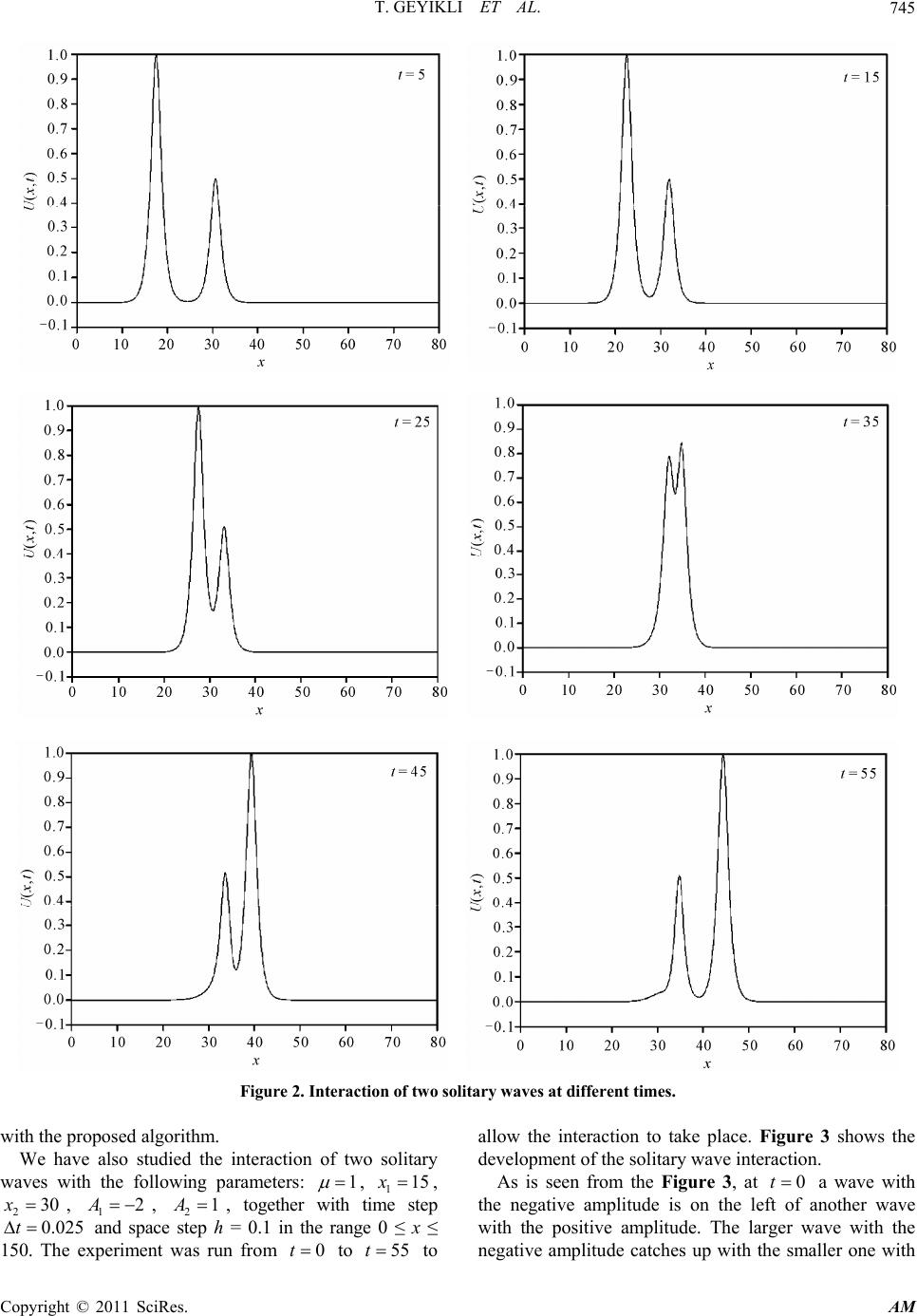 T. GEYIKLI ET AL.745 Figure 2. Interaction of two solitary waves at different times. with the proposed algorithm. We have also studied the interaction of two solitary waves with the following parameters: allow the interaction to take place. Figure 3 shows the development of the solitary wave interaction. As is seen from the Figure 3, at a wave with the negative amplitude is on the left of another wave with the positive amplitude. The larger wave with the negative amplitude catches up with the smaller one with 1 , 115x , ime step ≤ x ≤ 55 230x 0.02t 150. The 0t , , together with t t from 12A 5 and space ste xper ime n 21A, p h was run = 0.1 in the range 0 0 to e tt to Copyright © 2011 SciRes. AM 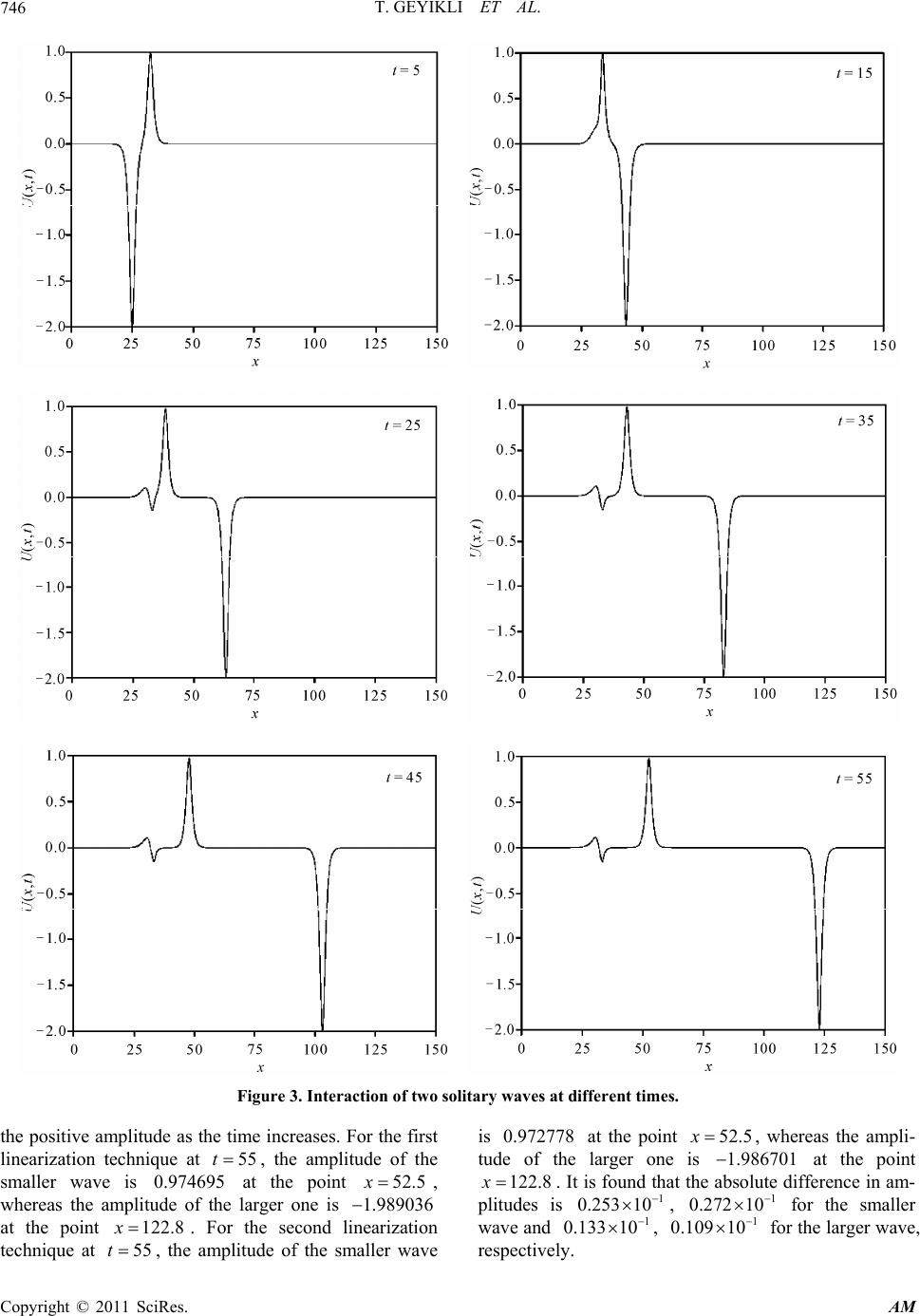 T. GEYIKLI ET AL. 746 Figure 3. Interaction of two solitary waves at different times. the positive amplitude as the time increases. For the first linearization technique at, the amplitude of the smaller wave is the point 55t 5 at 0.97469 52.5x , whereas the amr one is at the point e seco technique athe sm is at the point , whereas the ampli- arger on at the point plitude of t 122.8 , the am he large . For th plitude of t nd linea 1.989036 rization aller wave x 55t 0.972778 tude of the l 122.8 52.5x e is 1.986701 x . It is found th difference in am-at the absolute plitudes is 1 0.25310 1 13310 , for the smaller 1 0.272 10 wave and 0. , 1 10910 0. for the larger wave, respectively. Copyright © 2011 SciRes. AM  T. GEYIKLI ET AL.747 The analytical invariants by using Equation (1) can be found as , he invari- wellian initial condition breaks up into more solitary waves which were drawn in Figures 4(c)-(f) at time 12 3.1415927, 13.3333333CC 66667 . Table 3 lists the values of t ants of the two solitary waves with amplitudes 322.66C 12A , d for the the computer 21A. inva It can be seen that the values obtaine riants are satisfactorily constant during run. 8. The Maxwellian Initial Condition As a last study, we consider here is the numerical solu- tion of the Equation (1) with the Maxwellian initial con- dition 2 ,0 e Ux (14) with the boundary conditions 20,20,20,20, 0. xx UtUtUtUt As it is known, Maxwellian initial condition (14) the behavior of the solution, deends on the values of p . So we have considered various values for . For ases the first linearization technique the computations are carried out for the c1,0.5,0.1,0.05,0.02 and 0.005 which are used in the earlier papers [5,14]. When 1, 0.5 is used as shown Figures 4(a) and (b) at time 12t the Maxwellian initial condition does not cause development into a clean solitary wave. However with smaller valu0.1 es of ,0.05,0.02 and 0.005 Max- Table 3. Invariants for interaction of two solitary wave. 12 2, 1AA t Lineerization 1 C 2 C 3 C 0 −3.141573913.3332981 22.6665313 5 −3.137332413.3219118 22.6210653 15 −3.122709713.2806152 22.4483653 .3589494 −3.089663813.1922565 22.0973499 0 −3.1415739 13 13.3196543 22.6120524 15 −3.132507613.2805526 22.463773 3.113721013.1745553 8880 25 −3.114333713.2581754 22 First 35 −3.106033413.2359744 22.2706624 45 −3.097810613.2140028 22.1834701 55 .3332981 22.6665313 5 −3.1391704 3 25 −3.127738813.2535359 22.3561477 35 −3.123013813.2268810 22.2501653 45 −3.118341613.2005566 22.1457584 55 Second −22.042 12t . The numerical conserved quantities with 1,0.5,0.1,0.05,0.02 and are given in Tabl e 4. It is observed that the obtained values of the invariants remain almost constant during the computer run. Table 4. Invariants for Maxwellian initial condition, differ- ent µ. 0.005 t 1 C 2 C 3 C 0 1.772454 2.506607 0.886227 3 1.772972 2.506836 0.886561 6 1.775116 2.512628 0.890240 2.514942 0.891795 12 1 1.776698 2.515136 0.891967 3 9 1.772451 1.879967 0.886223 0 1.772454 1.46 0.886226 3 1.7724 1.37850.88614 6 9 0.1 0.05 0 9 1.721.1 12 1.710490 1.162646 0.737751 9 1.776365 0 1.772454 1.879971 0.886227 1.772452 1.879970 0.886225 6 1.772451 1.879968 0.886224 0.5 12 1.772450 1.879966 0.886222 3786 2091 7 1.772368 1.378507 0.886054 1.772316 1.378424 0.885933 12 1.772264 1.378340 0.885813 0 1.772454 1.315980 0.886227 3 1.772266 1.315654 0.885789 6 1.771976 1.315150 0.884947 9 1.771685 1.314648 0.884107 12 1.771396 1.314147 0.883270 1.772454 1.278380 0.886227 3 1.770834 1.275265 0.880933 6 1.768546 1.271572 0.874402 9 1.766186 1.266707 0.864400 12 0.02 1.763931 1.262351 0.855782 0 1.772454 1.259581 0.886227 3 1.757684 1.254254 0.928815 6 1.738212 1.227138 0.880527 2397 71836 0.714373 0.005 Copyright © 2011 SciRes. AM  T. GEYIKLI ET AL. Copyright © 2011 SciRes. AM 748 (a) b) ( (c) (d) (e) (f) Figure 4. Maxwellian initial condition, state at time t = 12 (a) µ = 1, (b) µ = 0.5, (c) µ = 0.1, (d) µ = 0.05, (e) µ = 0.02, (f) µ = 0.005.  T. GEYIKLI ET AL.749 9. Conclusions In this study, a numerical solution of the MEW equation based on the septic B-spline finite element has been pre- sented with three different linearization techniques. Three test problems are worked out to examine the per- formance of the algorithms. The performance and accu- racy of the method were demonstrated by calculating the error norms and on the motion of a single solitary wave. For the first and second linearization tech- niques, the error norms are sufficiently small and the invariants are satisfactorily constant in all computer run. The obtained results from the first and the second lin- earization techniques are almost the same and the com- puted results show that the present method is a remarka- bly successful numerical quation and can also be efficiently applied to other types of non-linear problem. 10. References [1] P. J. Morrison, J. D. Meiss and J. R. Carey, “Scattering of Regularized-Long-Wave Solitary Waves,” Physica D: Non- linear Phenomena, Vol. 11, No. 3, 1984, pp. 324-336. doi:10.1016/0167-2789(84)90014-9 [8] A. Esen, “A Numerical Solution of the Equal Width Wave Equation by a Lumped Galerkin Method,” Applied Mathematics and Computational, Vol. 168, No. 1, 2005, pp. 270-282. doi:10.1016/j.amc.2004.08.013 [9] A. Esen, “A Lumped Galerkin Method for the Numerical Solution of the Modified Equal Width Wave Equation Using Quadratic B Splines,” International Journal of Computer Mathematics, Vol. 83, No. 5-6, 2006, pp. 449- 459. doi:10.1080/00207160600909918 [10] B. Saka, “Algorithms for Numerical Solution of the Mo- dified Equal Width Wave Equation Using Collocation Method,” Mathematical and Computer Modelling, Vol. 45, No. 9-10, 2007, pp. 1096-1117. doi:10.1016/j.mcm.2006.09.012 2 L L [11] B. Saka and İ. Dag, “Quartic B-Spline Collocation Meth- od to the Numerical Solutions of the Burgers Equatio” Vol. 32, No. 3, May 2007, haos.2005.11.037 technique for solving the MEW e [2] L. R. T. Gardner and G. A. Gardner, “Solitary Waves of the Regularized Long Wave Equation,” Journal of Com- putational Physics, Vol. 91, No. 2, 1990, pp. 441-459. doi:10.1016/0021-9991(90)90047-5 [3] L. R. T. Gardner and G. A. Gardner, “Solitary Waves of the Equal Width Wave Equation,” Journal of Computa- tional Physics, Vol. 101, No. 1, 1992, pp. 218-223. doi:10.1016/0021-9991(92)90054-3 [4] L. R. T. Gardner, G. A Amein, “Simulations o I)1099-0887(199707)13:7<583::AID-C . Gardner, F. A. Ayoup and N. K. f the EW Undular Bore,” Commu- nications in Numerical Methods in Engineering, Vol. 13, No. 7, 1997, pp. 583-592. doi:10.1002/(SIC NM90>3.0.CO;2-E [5] S. I. Zaki, “Solitary Wave Interactions for the Modified Eual Width Equation,” Computer Physics Communica- tions, Vol. 126, No. 3, 2000, pp. 219-231. doi:10.1016/S0010-4655(99)00471-3 [6] S. I. Zaki, “A Least-Squares Finite Element Scheme for the Ew Equation,” Computer Methods in Applied Me- chanics and Engineering, Vol. 189, No. 2, 2000, pp. 587- 594. doi:10.1016/S0045-7825(99)00312-6 [7] A. M. Wazwaz, “The tanh and sine-cosine Methods for a Reliable Treatment of the Modified Equal Width Equa- tion and Its Variants,” Communications in Nonlinear Science and Numerical Simulation, Vol. 11, No. 2, 2006, pp. 148-160. doi:10.1016/j.cnsns.2004.07.001 n, Chaos, Solitons and Fractals, pp. 1125-1137. doi:10.1016/j.c [12] J. F. Lu, “He’s Variational Method for the Modified Equal Width Wave Equation,” Chaos, Solitons and Frac- tals, Vol. 39, No. 5, 2009, pp. 2102-2109. doi:10.1016/j.chaos.2007.06.104 [13] S. Hamdi, W. E. Enright, W. E. Schiesser, J. J. Gottlieb and A. Alaal, “Exact Solutions of the Generalized Equal Width Wave Equation,” Proceedings of the International Conference on Computational Science and Its Applica- tion, LNCS, Springer-Verlog, Berlin, Vol. 2668, 2003, pp. 725-734. [14] D. J. Evans, K. R. Raslan and A. Alaal, “Solitary Waves for the Generalized Equal Width (Gew) Equation,” In- ternational Journal of Computer Mathematics, Vol. 82, No. 4, 2005, pp. 445-455. [15] T. Geyikli, “Modelling Solitary Waves of a Fifth-Order Non-Linear Wave Equation,” International Journal of Computer Mathematics, Vol. 84, No. 7, July 2007, pp. 1607012943681079-1087. doi:10.1080/00207 TR R-436, Washington, DC, 1975. mber,” Applied Mathematical Modelling, Vol. 6, No. 5, October 1982, pp. 381-386. 07-904X(82)80102-9 [16] S. G. Rubin and R. A. Graves, “A Cubic Spline Ap- proximation for Problems in Fluid Mechanics,” NASA [17] J. Caldwell and P. Smith, “Solution of Burgers’ Equation with a Large Reynolds Nu doi:10.1016/S03 8] A. Esen and S. Kutluay, “Solitary Wave Solutions of the [1 Modified Equal Width Wave Equation,” Communications in Nonlinear Science and Numerical Simulation, Vol. 13, No. 8, 2008, pp. 1538-1546. doi:10.1016/j.cnsns.2006.09.018 [19] K. R. Raslan, “Collocation Method Using Cubic B-Spline for the Generalized Equal Width Equation,” International Journal of Simulation and Process Modelling, Vol. 2, No. 1-2, 2006, pp. 37-44. Copyright © 2011 SciRes. AM
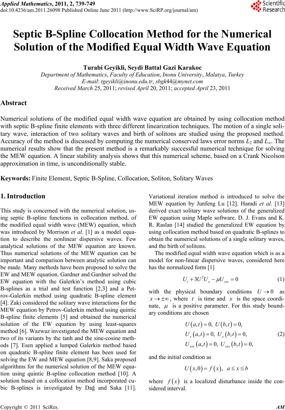
|