Applied Mathematics, 2011, 2, 732-738
doi:10.4236/am.2011.26097 Published Online June 2011 (http://www.SciRP.org/journal/am)
Dynamics of a Heroin Epidemic Model with Very
Population
Xiaoyan Wang1, Junyuan Yang1, Xuezhi Li2
1Department of Applied Mathematics, Yuncheng University, Yuncheng, China
2Department of Mat hem at i cs, Xinyang Normal University, Xinyang, China
Received March 26, 2011; revised April 16, 2011; accepted April 19, 2011
Abstract
Based on the model provided by the Mulone and Straughan [1], we relax the population which are constant
and obtain the drug-free equilibrium which is global asymptotically stable under some conditions. The sys-
tem has only uniqueness positive endemic equilibrium which is globally asymptotically stable by using the
second compound matrix.
Keywords: Heroin Epidemic Model, Equilibrium, Global Stability
1. Introduction
Heroin is an opiate drug that is synthesized from mor-
phine, a naturally occurring substance extracted from the
seed pod of the Asian opium poppy plant. Heroin usually
appears as a white or brown powder or as a black sticky
substance, known as “black tar heroin” [2]. Heroin users
are at high risk for addiction—it is estimated that about
23 percent of individuals who use heroin become de-
pendent on it. The spread of heroin habituation and ad-
diction presents many of the well-known phenomena of
epidemics, including rapid diffusion and clear geo-
graphic boundaries. It is unrealistic to repeat the experi-
ment on the human body for obtaining the statistic data.
Mathematical models play very important role in dealing
with these problems. Mathematical modellings are very
useful tools to predict how classes of drug takers behave,
and provide a good suggestion for the treatment strate-
gies. It is interest to explore the problem mathematically,
reducing the factors to the essential transmission mecha-
nism, in real life, is much more complex because of im-
ponderable and often intervening biological, psycho-
logical, and social conditions.
During recent years, many mathematical models have
been developed to describe the Heroin epidemic model
(see [1,3]). One of the recent model divided the mathe-
matical problem into tree class, namely susceptibles,
heroin users or alcoholics, and heroin users or alcoholics
undergoing treatment which denote by



1
, StU t
and , respectively. The model is

2
Ut


11
312 111
11
312 2
12
d,
d
dδ,
d
dδ
d
SU
SS
tN
UU
USU p
tN N
UU
UpU U
tN 2
U






 
 
(1.1)
where the number of individuals enter the susceptible
population at a rate,

, die at rate

. Infection of a
drug user occurs through a simple mass action process
11
SU N

, where 1

is probability of becoming a drug
user, per unit time. The probability of a drug user in
treatment relapsing to untreated use, per unit time is .
Infected heroin users die at enhanced rate 1, treatment
infected heroin users die at enhanced rate 2. In this
model, the authors considered the global stability of the
drug equilibrium under some conditions. However, they
treated the total population is a constant for simple. In
fact, we sum the tree equations of (1.1) and get
p
δ
δ
112 2
dδδ.
d
NNU U
t
 
It is easy to see that the total population is not a con-
stant. This assumption is not reasonable and maybe sim-
ply the problem. Since (1.1) can be changed a plane sys-
tem under the constant population. In our paper we will
relax this assumption and assume the total population is
very according to the time. In our model we use the bi-
linear law incidence function instead of standard inci-
dence. The model is changed into

X. Y. WANG ET AL.733


11
1
11 31211
2
1312 22
d,
d
dδ,
d
dδ
d
SSU S
t
USUU UpU
t
UpUUUU
t

 


 
 
(1.2)
2. Basic Reproduction Number and Stability
of Drug-Free Equilibrium
The drug-free equilibrium is given by

0
0,0,0,0,0.ES

 



The basic reproduction number 0 is defined to be
the expected number of secondary cases produced, in a
completely susceptible population, by a typical infected
individual during its entire period of infection. We fol-
low the recipe of [4] to calculate the basic reproduction
number. O. Diekmann et al. in [5] has shown 0 as the
spectral radius of the next generation matrix. Firstly we
need to separate the new infections from other factors.
We define
R
R

F
X to be the vector which represents the
rate of new infections that appear in the population
where
X
is a vector given by

12
,,

X
UU S. In this
model, we get ,

11
,0,0FSU  
 
 
31211 312
22 111
δ,
δ,
VUUp UUU
UpUUSS


 
 
,
F
V have the same definition as explained in [4].
According to the recipe presented in [4] we define the
derivatives and in the following
way

0
DF E

0
DV E
100
000
000
F






 



and
1
2
1
δ00
δ0.
0
p
Vp









  










Finally the basic reproduction number is obtained by
calculating the spectral radius of 1
F
V. Then the basic
reproduction number for the model presented in system
(1.2) is given by the following expression


11
0
1
.
δ
RFV p





This completes the calculation of basic reproduction
number. The Jacobian matrix of (1.2) at drug-free equi-
librium is
0
E


0
1
1
1
2
0
0δ0
0δ
E
Jp
p



















The characteristic roots of the matrix are
 
1
1223
0, δ0, δ.p

 


 1
Hence the characteristic equation just has negative real
part roots under some condition. Then we can obtain the
following theorem.
Theorem 2.1. If 01R

, the drug-free equilibrium is
locally asymptotically stable otherwise it is unstable.
Theorem 2.2. If

1
1
1
δ



 drug-free equilibrium
is globally stable.
Proof. We set a Lyapunov function


121 2
,,VtUUU U

.
Then



 
12
21
11112 2
1
11
1
d
d
δδ
δ1δ
δ
VUU
t
SU UU
UU
 








 




22
When

1
1
1
δ




, it is easy to get d0
d
V
t

. Also
0V

 if and only if are all zero. Note that the
12
,UU
largest invariant set is d
,0,0 0
d
V
Mt



 



 

, the
drug-free equilibrium 0 is globally asymptotically
stable by Lassale’s invariance principle.
E
3. Existence and Stability of the Endemic
Equilibrium
In this section we discuss the existence of the endemic
equilibrium. We just consider the special situation. We
find the positive endemic equilibrium for (1.2) which is
obtained by solving the following sets of equations

X. Y. WANG ET AL. 734
From the expression of 1 and 2
U, and positivity
of the endemic equilibrium, we note that
U 


11
11 32311
1312 22
0,
δ0,
δ0.
SU S
SUUU pU
pUU UU

 

 
 
 
 






(3.1)
*1
1
δ
min, p S




 




Solving the first and second equations of (3.1), we ob-
tain If ,
01R1
1
δp
S





. We assume the two real
1
12
3 1
δ
,p
S
UU
S









. Substituting 1 U

and
positive roots of (1.2) are respectively
x
 and
x

, we
check the positive real roots of (1.2)
2 into the third equation of (3.1), we obtain
US

should satisfies the following equation
.

20AxBx C P E
x
Number of Real Positive Roots of (3.1)
1
1
δp
x





 1
1
1
δp
x





 0
where



2
1213
1331 121
31
,
δδ,
.
A
Bp
C
 



 
 

δ (3.2)
In our model, we just consider 13

 

PE
. It is easy to
see and . Due to Descarters’ rule of sings,
the number of real positive roots of is deter-
0A0C


Concluding the above discussion, then we can obtain
the following theorem.
Theorem 3.1. 1) If , and
01R1
1
δp
x




, (1.2)
mined by the following table
B Number of Real Positive Roots
>0 1
<0 1
has only unique real positive endemic equilibrium.
Next, we will discuss the locally stability of the en-
demic equilibrium. The Jacobian matrix at endemic equi-
librium is


11 1
1113 2131
32312
0
δ.
0δ
E
US
JUSUp U
pU U
 
 



 


 








Then the characteristic of the endemic equilibrium is
32
123
0,aaa    (3.3)
where
 
 

  
131 111
211312311113 1
2
33111111311 12
2δ0
δδ 0,
δδ0.
aU U
aU UUSU
aUUSU SU

 
 

 
 

 

Define

12 3
,
H
Eaaa

and straightly calculate and then we obtain
  


22
31 21131 2112321111
δδδ .HEUUUUUSUU


 

 



Define

11 ,yU


 and




31 22 32
δδ.
2
f
yy U 



2


Theorem 3.2. Let E

be the endemic equilibria of
system (1.2) as defined before, and assume
U    Note that

31 2232
δ4δ0,UU    

it is easy to 1
1
δp
x





 and , then it is locally asympto-
01R
get . Due to the Routh Hurtwiz [6], we get
the following theorem.

0HEtically stable.

X. Y. WANG ET AL.735
Finally, we will consider the global stability of the
endemic equilibrium is asymptotically orbitally stable
with asymptotic phase.
Theorem 3.3. The endemic equilibrium of E

to
(1.2), if it exists, is asymptotically orbitally stable with
asymptotic phase.
Proof. The second compound matrices


12
,,
J
SU U
of (1.2) is given by


1113 2
31
1
3211 3121
13231
11
12
0
2δ
(2 δ),
02δδ
USU U
p
pUU US
SU U
Up
 

 
 






 












 


we can write the linear system (1.2) with respect to a
solution of (1.2) as the following
system (3.4):
  
12
,,St U t Ut


33




11113 231
3213 121
111213 231
2δ,
2δ,
2δδ .
X
UpSUXUY
YpUXU YSZ
Z
UYpSUUZ




 


To show the asymptotic stability of the system (3.4)
we consider the following function:

12 12
,,;, ,, ,,,V XYZSUUPSUUXYZ


where the matrix


1212
,,P diagIUUUU and

is the norm in defined by
3
R




,,sup ,.
X
YZXYz
(3.5)
Suppose that the solution
 

 
12
,,St U t Ut
P is pe- riodic of least period . The matrix and its in-
verse are thus well defined and smooth along
0w

. There
exists constant such that 0c

12
(,,;, ,),,VXYZSUUc XYZ. (3.6)
for all


3
,,
X
YZ R and

,,SEI

. Let








,,
X
tYtZt be a solution to (3.4) and
  
1
12
2
,,;,,) sup,.
U
Vt VXYZSUUXY z
U





The right-hand derivative of


Vt exists and its calcu-
lation is described in [7]. In fact, direct calculation yields



1
11113 231
2
2δ,
U
DXtUpSU XUYz
U



 


and



 
3213121
111213 231
2δ,
2δδ .
DYpUXUYSZ
DZUYpSUU Z








and thus
  
  
12
111
21222
12
11
32312 32
2212
,
2δ.
UUU
UU
DYzYz DYz
UUUUU
UU
UU
pUXYzUUYz
UUUU




 




 



We claim that


 
12
sup ,DV tgtgtV t

where


11111
12
231
12
2δ
2δ
gtU pS
UU
232
g
tU
UU


 

 U
Using (1.2), we find

11
11132
11
,
UU
gtU U
UU





 
and

1
2
2
0
pU
gt U


and thus
   
12 1
0 0sup,d log0
ww
gtgttUtw  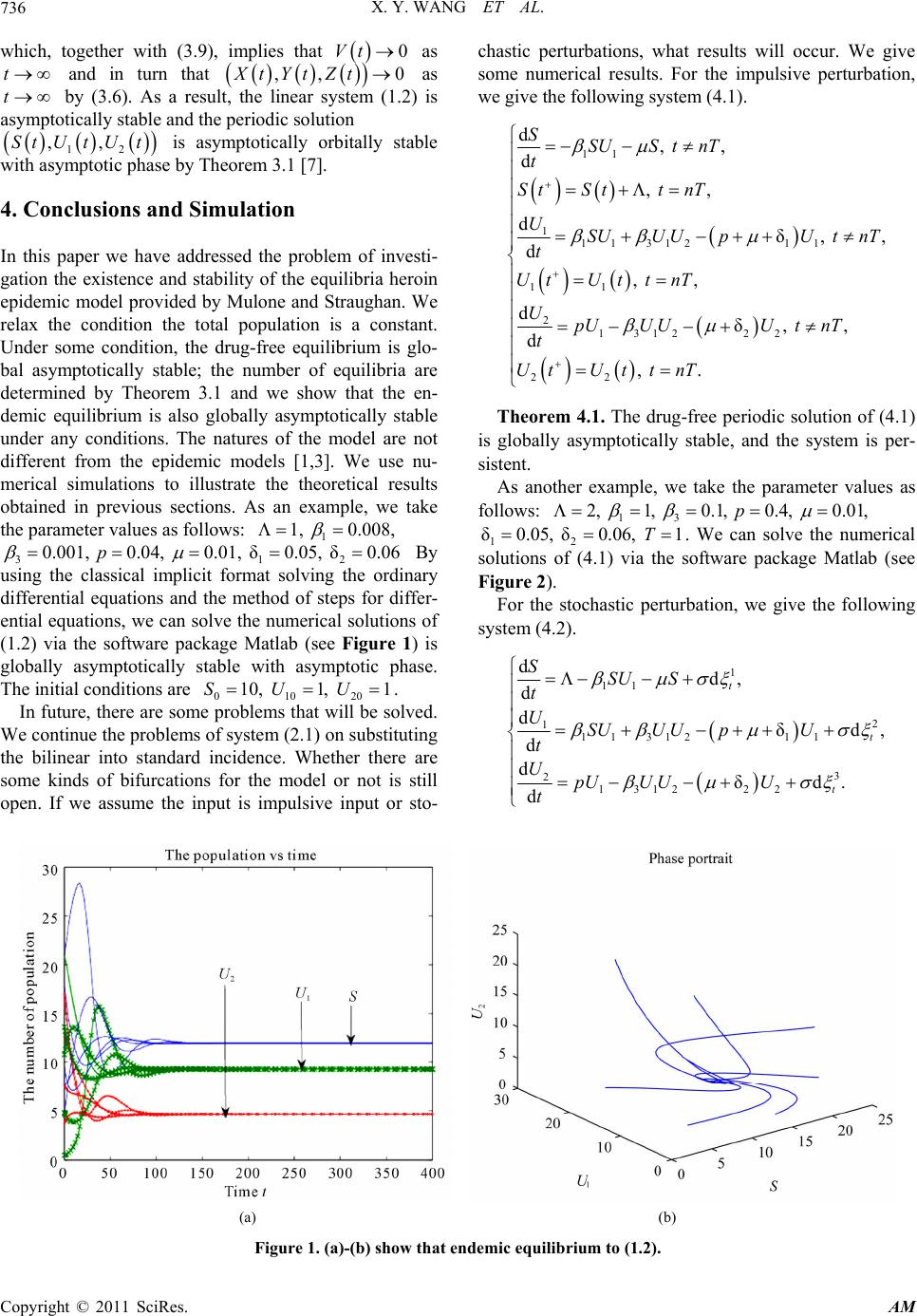


X. Y. WANG ET AL. 736
which, together with (3.9), implies that as
and in turn that

0Vt

t
 


Zt,,Xt Yt

0 as
by (3.6). As a result, the linear system (1.2) is
asymptotically stable and the periodic solution
12
is asymptotically orbitally stable
with asymptotic phase by Theorem 3.1 [7].
t

St
 

,,UtUt
4. Conclusions and Simulation
In this paper we have addressed the problem of investi-
gation the existence and stability of the equilibria heroin
epidemic model provided by Mulone and Straughan. We
relax the condition the total population is a constant.
Under some condition, the drug-free equilibrium is glo-
bal asymptotically stable; the number of equilibria are
determined by Theorem 3.1 and we show that the en-
demic equilibrium is also globally asymptotically stable
under any conditions. The natures of the model are not
different from the epidemic models [1,3]. We use nu-
merical simulations to illustrate the theoretical results
obtained in previous sections. As an example, we take
the parameter values as follows: 1 1, 0008,

 
δ005, δ006
312
0001, 004, 001,p

  
10
 
, 1, 1SU U
By
using the classical implicit format solving the ordinary
differential equations and the method of steps for differ-
ential equations, we can solve the numerical solutions of
(1.2) via the software package Matlab (see Figure 1) is
globally asymptotically stable with asymptotic phase.
The initial conditions are 01020

.
In future, there are some problems that will be solved.
We continue the problems of system (2.1) on substituting
the bilinear into standard incidence. Whether there are
some kinds of bifurcations for the model or not is still
open. If we assume the input is impulsive input or sto-
chastic perturbations, what results will occur. We give
some numerical results. For the impulsive perturbation,
we give the following system (4.1).








11
1
11 31211
11
2
1312 22
22
d, ,
d
, ,
dδ, ,
d
, ,
dδ, ,
d
, .
SSUS tnT
t
StStt nT
USUUUpUtnT
t
UtUttnT
UpUUUUtnT
t
UtUt tnT

 




  




 




 




Theorem 4.1. The drug-free periodic solution of (4.1)
is globally asymptotically stable, and the system is per-
sistent.
As another example, we take the parameter values as
follows: 13 2, 1, 01, 04, 001,p



 
T
12
δ005, δ006, 1

. We can solve the numerical
solutions of (4.1) via the software package Matlab (see
Figure 2).
For the stochastic perturbation, we give the following
system (4.2).


1
11
2
1
11 31211
3 2
1312 22
dd,
d
dδd,
d
dδd.
d
t
t
t
SSU S
t
USUUUpU
t
UpUUUU
t



 
 


 


 



(a) (b)
Figure 1. (a)-(b) show that endemic equilibrium to (1.2).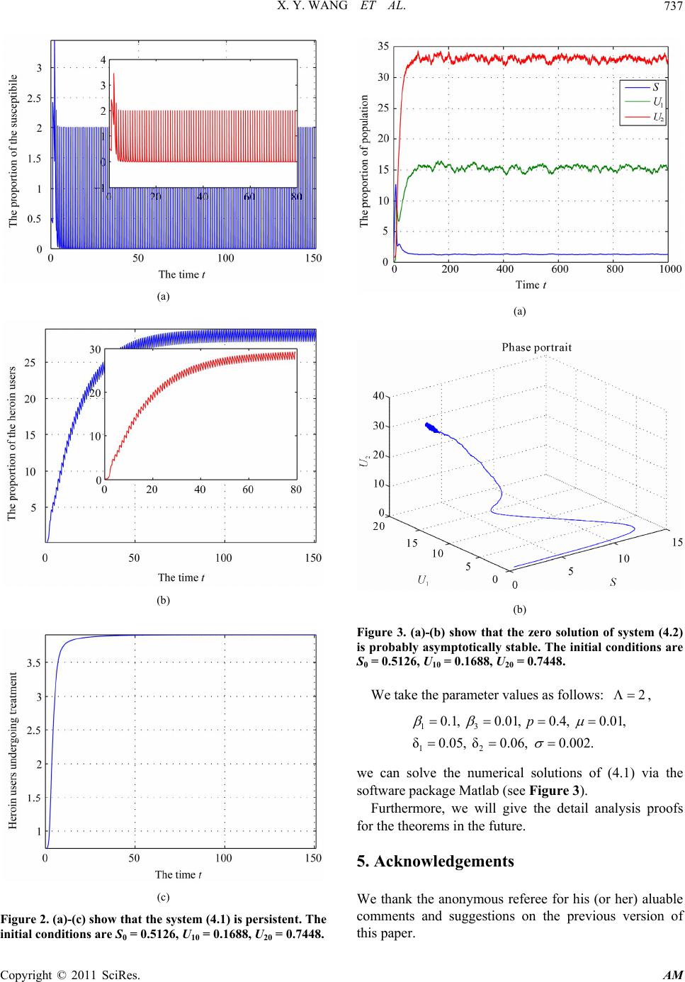

X. Y. WANG ET AL. 737
(a)
(b)
(c)
Figure 2. (a)-(c) show that the system (4.1) is persistent. The
initial conditions are S0 = 0.5126, U10 = 0.1688, U20 = 0.7448.
(a)
(b)
Figure 3. (a)-(b) show that the zero solution of system (4.2)
is probably asymptotically stable. The initial conditions are
S0 = 0.5126, U10 = 0.1688, U20 = 0.7448.
We take the parameter values as follows: , 2
13
12
01, 001, 04, 001,
δ005, δ006, 0002.
p 



 
we can solve the numerical solutions of (4.1) via the
software package Matlab (see Figure 3).
Furthermore, we will give the detail analysis proofs
for the theorems in the future.
5. Acknowledgements
We thank the anonymous referee for his (or her) aluable
comments and suggestions on the previous version of
this paper.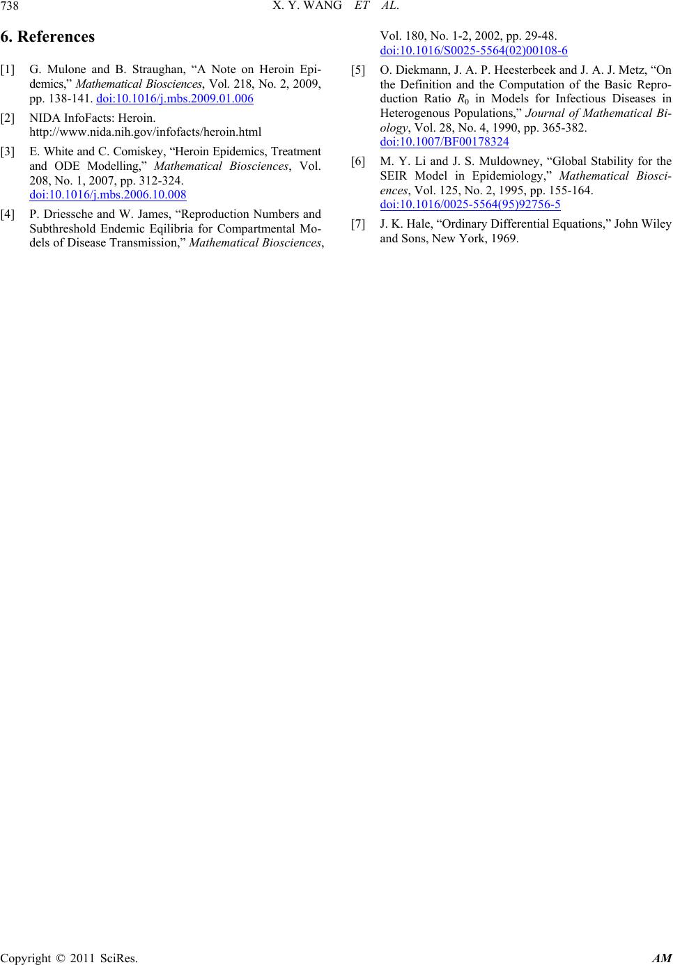

X. Y. WANG ET AL. 738
6. References
[1] G. Mulone and B. Straughan, “A Note on Heroin Epi-
demics,” Mathematical Biosciences, Vol. 218, No. 2, 2009,
pp. 138-141. doi:10.1016/j.mbs.2009.01.006
[2] NIDA InfoFacts: Heroin.
http://www.nida.nih.gov/infofacts/heroin.html
[3] E. White and C. Comiskey, “Heroin Epidemics, Treatment
and ODE Modelling,” Mathematical Biosciences, Vol.
208, No. 1, 2007, pp. 312-324.
doi:10.1016/j.mbs.2006.10.008
[4] P. Driessche and W. James, “Reproduction Numbers and
Subthreshold Endemic Eqilibria for Compartmental Mo-
dels of Disease Transmission,” Mathematical Biosciences,
Vol. 180, No. 1-2, 2002, pp. 29-48.
doi:10.1016/S0025-5564(02)00108-6
[5] O. Diekmann, J. A. P. Heesterbeek and J. A. J. Metz, “On
the Definition and the Computation of the Basic Repro-
duction Ratio R0 in Models for Infectious Diseases in
Heterogenous Populations,” Journal of Mathematical Bi-
ology, Vol. 28, No. 4, 1990, pp. 365-382.
doi:10.1007/BF00178324
[6] M. Y. Li and J. S. Muldowney, “Global Stability for the
SEIR Model in Epidemiology,” Mathematical Biosci-
ences, Vol. 125, No. 2, 1995, pp. 155-164.
doi:10.1016/0025-5564(95)92756-5
[7] J. K. Hale, “Ordinary Differential Equations,” John Wiley
and Sons, New York, 1969.