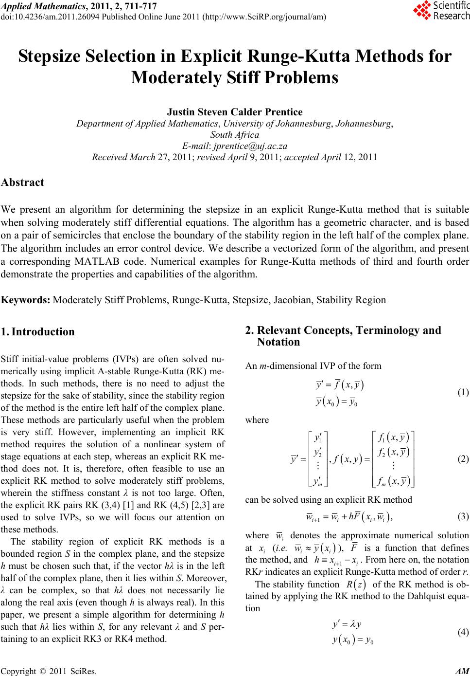
Applied Mathematics, 2011, 2, 711-717
doi:10.4236/am.2011.26094 Published Online June 2011 (http://www.SciRP.org/journal/am)
Stepsize Selection in Explicit Runge-Kutta Methods for
Moderately Stiff Problems
Justin Steven Calder Prentice
Department of Applied Mathematics, University of Johannesburg, Johannesburg,
South Africa
Received March 27, 2011; revised April 9, 2011; accepted April 12, 2011
Abstract
We present an algorithm for determining the stepsize in an explicit Runge-Kutta method that is suitable
when solving moderately stiff differential equations. The algorithm has a geometric character, and is based
on a pair of semicircles that enclose the boundary of the stability region in the left half of the complex plane.
The algorithm includes an error control device. We describe a vectorized form of the algorithm, and present
a corresponding MATLAB code. Numerical examples for Runge-Kutta methods of third and fourth order
demonstrate the properties and capabilities of the algorithm.
Keywords: Moderately Stiff Problems, Runge-Kutta, Stepsize, Jacobian, Stability Region
1. Introduction
Stiff initial-value problems (IVPs) are often solved nu-
merically using implicit A-stable Runge-Kutta (RK) me-
thods. In such methods, there is no need to adjust the
stepsize for the sake of stability, since the stability region
of the method is the entire left half of the complex plane.
These methods are particularly useful when the problem
is very stiff. However, implementing an implicit RK
method requires the solution of a nonlinear system of
stage equations at each step, whereas an explicit RK me-
thod does not. It is, therefore, often feasible to use an
explicit RK method to solve moderately stiff problems,
wherein the stiffness constant λ is not too large. Often,
the explicit RK pairs RK (3,4) [1] and RK (4,5) [2,3] are
used to solve IVPs, so we will focus our attention on
these methods.
The stability region of explicit RK methods is a
bounded region S in the complex plane, and the stepsize
h must be chosen such that, if the vector hλ is in the left
half of the complex plane, then it lies within S. Moreover,
λ can be complex, so that hλ does not necessarily lie
along the real axis (even though h is always real). In this
paper, we present a simple algorithm for determining h
such that hλ lies within S, for any relevant λ and S per-
taining to an explicit RK3 or RK4 method.
2. Relevant Concepts, Terminology and
Notation
An m-dimensional IVP of the form



00
,yfxy
yx y

 (1)
where




11
22
,
,
,,
,
mm
y
f
xy
y
f
xy
yfxy
y
f
xy

 





 


 



(2)
can be solved using an explicit RK method

1, ii ii
wwhFxw


, (3)
where i w denotes the approximate numerical solution
at i
x
(i.e.


ii
wyx),
F
is a function that defines
the method, and 1ii hx x


. From here on, the notation
RKr indicates an explicit Runge-Kutta method of order r.
The stability function


Rz of the RK method is ob-
tained by applying the RK method to the Dahlquist equa-
tion

00
yy
yx y



 (4)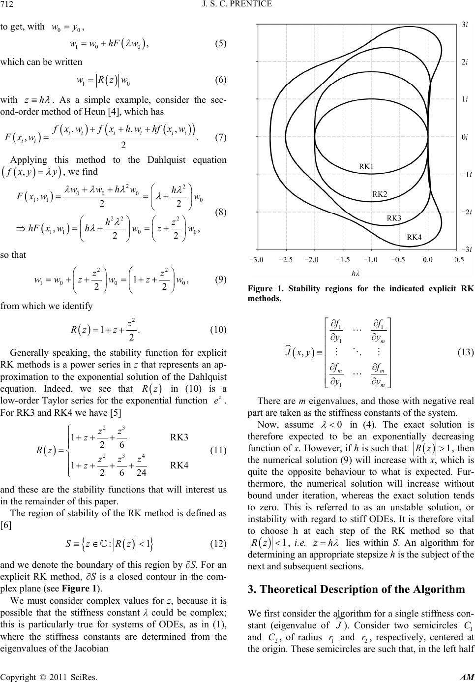

J. S. C. PRENTICE 712
to get, with ,
00
wy


10 0
,wwhFw   (5)
which can be written

1
wRzw0 (6)
with zh

. As a simple example, consider the sec-
ond-order method of Heun [4], which has

 


,,
,.
2
iii iii
ii
fxwfxhw hfxw
Fxw  ,
(7)
Applying this method to the Dahlquist equation
 
,
f
xy y

, we find


22
00 0
11 0
22 2
110 0
,22
,,
22
wwhw h
F
xw w
hz
hF x whwzw
 












(8)
so that
22
10 00
1,
22
z
ww zwzw

 


z
(9)
from which we identify

2
1
2
z
Rz z .
(10)
Generally speaking, the stability function for explicit
RK methods is a power series in z that represents an ap-
proximation to the exponential solution of the Dahlquist
equation. Indeed, we see that in (10) is a
low-order Taylor series for the exponential function

Rz
z
e.
For RK3 and RK4 we have [5]

23
234
1
26
1
2624
zz
z
Rz zzz
z
 



 


RK3
RK4
(11)
and these are the stability functions that will interest us
in the remainder of this paper.
The region of stability of the RK method is defined as
[6]


:Sz Rz 

1 (12)
and we denote the boundary of this region by ∂S. For an
explicit RK method, ∂S is a closed contour in the com-
plex plane (see Figure 1).
We must consider complex values for z, because it is
possible that the stiffness constant λ could be complex;
this is particularly true for systems of ODEs, as in (1),
where the stiffness constants are determined from the
eigenvalues of the Jacobian
Figure 1. Stability regions for the indicated explicit RK
methods.

11
1
1
,
m
mm
m
f
f
yy
Jxy
f
f
yy






















 

(13)
There are m eigenvalues, and those with negative real
part are taken as the stiffness constants of the system.
Now, assume 0


in (4). The exact solution is
therefore expected to be an exponentially decreasing
function of x. However, if h is such that

1Rz , then
the numerical solution (9) will increase with x, which is
quite the opposite behaviour to what is expected. Fur-
thermore, the numerical solution will increase without
bound under iteration, whereas the exact solution tends
to zero. This is referred to as an unstable solution, or
instability with regard to stiff ODEs. It is therefore vital
to choose h at each step of the RK method so that


1Rz

, i.e. zh


lies within S. An algorithm for
determining an appropriate stepsize h is the subject of the
next and subsequent sections.
3. Theoretical Description of the Algorithm
We first consider the algorithm for a single stiffness con-
stant (eigenvalue of
J


1
i
). Consider two semicircles 1
and , of radius and , respectively, centered at
C
half
2
C
orig
r2 r
circles are sthe in. These semuch that, in the left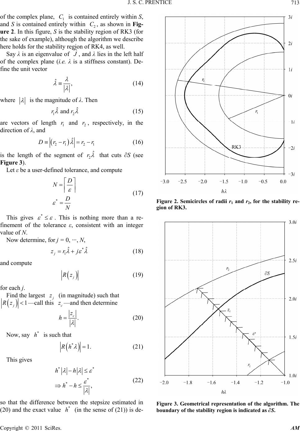

J. S. C. PRENTICE713
of the complex plane, 1 C is contained entirely within S,
and S is contained entirely within 2
C, as shown in Fig-
ure 2. In this figure, S is the stabiliegion of RK3 (for
the sake of example), although the algorithm we describe
here holds for the stability region of RK4, as well.
Say λ is an eigenvalue of
ty r
J

, and λ lies in the left half
of the complex plane (i.e. λ a stiffness constant). De-
fine the unit vector
is
ˆ,



 (14)
where

is the magnitude of λ. Then
12
ˆˆ
and rr

 (15)
are vectors of length and
1
r2 r, respectively, in the
direction of λ, and

2121
rr
2ˆ
r
ˆ
r    (16)
is the length of the segment of
Dr

that cuts ∂S (see
user-defined toleraompute
Figure 3).
Let ε be ance, and c
*
D
N
D
N





(17)
This gives

*

 
e toler
. This is noting more than a re-
fin
rmine, for j = 0, ···, N,
h
ement of thance ε, consistent with an integer
value of N.
Now dete
*
ˆˆ
zr j
1
j

  (18)
and compute

j
Rz (19)
for each j.
largest Find the
j
z (in magnitu such that de)

1z—call thc z—and then determine
j
Ris
.
c
z
h

 (20)
Now, say is such that
*
h

*
Rh 1.   (21)
This gives
**
*
,
*
hh
hh





 (22)
so that the difference between thpsize estimated in
(20) and the exact value (in the sense of (21)) is de-
e ste
*
h
Figure 2. Semicircles of radii r1 and r2, for the stability re-
gion of RK3.
Figure 3. Geometrical representation of the algorithm. The
boundary of the stability region is indicated as ∂S.

J. S. C. PRENTICE 714
pendent on *

 , and

. Hence, the smaller we
choose ε, the closer the endpoint of hλ is to ∂S, particu-
larly for large

.
Note the following: (22) gives
**
hh
1
h hhr

  


(23)
and if we demand that the relative difference
*
hh
h

must be less than some value δ, then choosing
1
r

1
r

  (24)
ensures that this will be case. In other words, (24) pro-
vides a form of error control, since 1 r and δ are known
a priori.
The algorithm is depicted in Figure 3. In this figure,
the curves labelled 1
r and 2 r are the semicircles, and
∂S indicates the boundary of the stability region. The
arrow touching the 1
r semicircle indicates 1ˆ
r

, and the
arrow touching the 2 r semicircle indicates 2ˆ r

. The
arrows between these two represent
j
z for
1, ,1jN. The separation of two adjacentws is
*
arro

, as indicated. The arrow within S and closest to ∂S is
It is clear that ∂S cuts 2ˆ
r
c
z, as shown.

. The segment
ween arrowheads that ∂S cuts is the segment of length
D, referred to earlier.
For a system of ODEs, in which there is more than one
stiffness constant, we
bet
would apply the above algorithm
for each such constant. This would yield a stepsize for
each stiffness constant, and we would choose the mini-
mum of these stepsizes as h in (3).
4. Implementation of the Algorithm
algorithm, H
c
ere we present a vectorized version of the
atering for a system of ODEs which has more than one
stiffness constant.
The parameters 12 ,rr and ε are input from which N
and *

are easily mined. Assume that the set of
eigenvalues of
deter

,
ii
J
xw
 yields M distinct stiffness con-
stants (note that
M
m). Let

denote a row vector
containing these ess constants, as in
M stiffn


12
,
M
 λ (25)
and let ˆ

denote the corresponding
n
vector of unit vec-
tors, as i

12
12
12
ˆ
.
M
M
M
 
 
 







λ
111
222
A
NN N


















(27)
12
12
12
ˆ
ˆ times




(28)
ˆ
M
M
M
LN

 

 

 

 

 

 
 

 









and hence, determine


*
1
1NM
Z
rA L  



where
(29)
1
N
M
ent-by
is the N × M unit matrix, and ⊠ denotes the
elem-element product of two matrices, sometimes
product (the matrices must have
f course). The structure of
known as the Hadamard
the same dimensions, o
Z

 is




**
1112 1
ˆˆ M
rr  


*
ˆ
r

 
 
** *
1112 1
** *
111 21
ˆˆ ˆ
22 2
.
ˆˆ
M
M
rr r
Z
rN rNrN
  
 



(26)
Define the N × M matrices
ˆ




 

 




 








(30)
We then evaluate

1 RK3
26
126
RK4
24
ZZZZZ
Z
ZZZZZ
RZ Z
ZZ

ZZ





 








  

 


where
 

(31)


RZ

 is an N × M matrix, of which the jkth en-
try is







*
1ˆ. k
jk
RZRrj

 

 (32)
We compute


RZ

 , the matrix containing the mag-
f eacnitude oh element of

RZ

, and we find the largest
entry less than unity in each column of

RZ
 . The cor-
responding elements in
Z

 are the for each stiffness
coare M
c
nstant. There such values of c
z, one for each
z
stiffness constant k

(denotehem ,ck z), and we de-
termine
t
,ck
z
k
k
h

 (33)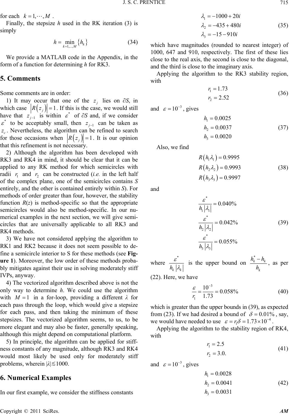

J. S. C. PRENTICE715
(34)
We provide a MATLAB code
nction for determining h for RK3.
5.
Some comments are in order:
1) It may occur that one of the
for each 1, ,kM.
Finally, the stepsize h used in the RK iteration (3) is
simply

1,...,
min k
kM
hh


in the Appendix, in the
form of a fu
Comments
j
z lies on ∂S, in
which case

1
j
Rz . If this is the case, we would still
have that 1
j
z is within *

of ∂S and, if we consider
*

to be acceptably small, then 1
j
z
can
 ca
be
n be taken as
gorefined to search
when
c
z. Nevertheless, the al
r those occasions
rithm
fo


1
j
Rz . It is our opinion
ssar
n
4 in mind
any
ad d
of

y. that this refinement is not nece
2) Although the algorithm has bee developed with
RK3 and RK, it should be clear that it can be
applied to RK method for which semicircles with
rii 1 r and 2 r can be constructe (i.e. in the left half
the complex plane, one of the semicircles contains S
entirely, and the other is contained entirely within S). For
methods of order greater than four, however, the stability
function R(z) is method-specific so that the appropriate
semicircles would also be method-specific. In our nu-
merical examples in the next section, we will give semi-
circles that are universally applicable to all RK3 and
RK4 methods.
3) We have not considered applying the algorithm to
RK1 and RK2 because it does not seem possible to de-
fine a semicircle interior to S for these methods (see Fig-
ure 1). Moreover, the low order of these methods proba-
bly mitigates against their use in solving moderately stiff
IVPs, anyway.
4) The vectorized algorithm described above is not the
only way to determine h. We could use the algorithm
with 1
M
 in a for-loop, providing a different λ for
each pass through the loop, which would give a stepsize
for each pass, and then taking the minimum of these
stepsizes. The vectorized algorithm seems, to us, to be
more elegant and may also be faster, generally speaking,
al
onstan
though this might depend on computational platform.
5) In principle, the algorithm can be applied for stiff-
ness cts of any magnitude, although RK3 and RK4
would most likely be used only for moderately stiff
problems, wherein |λ|≲1000.
6. Numerical Examples
In our first example, we consider the stiffness constants
1
2
3
1000 20
435 480
15 910
i
i
i





 

(35)
which have magnitudes (rounded to nearest integer) of
ly. The first of these lies
ose to the real axis, the second is close to the diagonal,
Applying the algorithm to the RK3 stability region,
with
(36)
1000, 647 and 910, respective
cl
and the third is close to the imaginary axis.
1
2
1.73
2.52
r
r


and 3 10 

, gives
1
2
0.0025
0.0037
h
h
30.0020h



(37)
Also, we find




11
22
33
0.9995
0.9993
0.9997
Rh
h
Rh






R (38)
and
*
11
*
22
*
33
0.040%
0.042%
0.055%
h
h
h









(39)
is the upper bound on
*
kk
k
hh
h

*
kk
h


where , as per
(22). Here, we have
3
1
10 0.058%
1.73 r


 (40)
which is greater than the upper bounds in (39), as expected
from (23). If we had desired a bound of 0.01%


73 10
, say,
havwe woulde needed to use 4
11.r


 . 
e stability region of RK4, Applying the algorithm to th
with
1
2
2.5
3.0.
r
r

 (41)
and 3 10 

, gives
1
2
0.0028
0.0
h
h
3
041
0.0031
h



(42)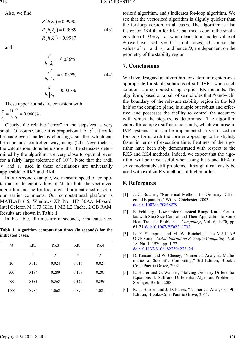

J. S. C. PRENTICE 716
and
torized algoritd f is foralgore
see that the vectorized algorithm is slightly quicker than
the for-loop v, in aorithmlso
fastr RK4for Rt thise to t
er value of
hm, anndicate-loop ithm. W
ersionll cases. The alg is a
er fo than K3, bu is duhe small-
21
Also, we find



11
22
33
0.9990
0.9987
Rh
Rh
Rh






0.9989 (43)
Dr r

,
e u 
which leads to a aller value of
N (v
sm
we hased 3

in 10all caf cothe
n algor
icircles that “sandwich”
relevant stability region in the left
plane, is simple but robust and effec-
ses). Ourse,
values of 1
r and 2 r, and hence D, are dependent on the
geometry of the stability region.
7. Conclusions
We have designed aithm for determining stepsizes
appropriate for stable solutions of stiff IVPs, when such
solutions are computed using explicit RK methods. The
gorithm, based on a pair of sem
*
11
*
22
*
33
0.036%
0.037%
0.035%
h
h
h









(44)
upper bounds are consistent with
al
the boundary of the
alf of the complex
These h
3
1
10 0.040%
2.5 r


 .
Clearly, the relative “error” in the stepsizes is very
small. Of course, since it is proportional to
tive, and possesses the facility to control the accuracy
with which the stepsize is determined. The algorithm
caters for complex stiffness constants, which can arise in
IVP systems, and can be implemented in vectorized or
for-loop form, with the former appearing to be slightly
faster in terms of execution time. Features of the algo-
rithm have been ably demonstrated with respect to the
RK3 and RK4 methods. Indeed, we expect that the algo-
rithm will be most useful when using RK3 and RK4 to
solve moderately stiff problems, although it can easily be
used with explicit RK methods of higher order.
8. References
[1] J. C. Butcher, “Numerical Methods for Ordinary Differ-
ential Equations,” Wiley, Chichester, 2003.
doi:10.1002/0470868279
2] E. Fehlberg, “Low-Order Classical Runge-Kut
*

, it could
maller, which can be made even smaller by choosing ε s
be done in a controlled way, using (24). rtheless,
the calculations done here show that the stedeter-
mined by the algorithm are very close to al, even
for a fairly large tolerance
universally
applicable to RK3 and RK4.
In our second example, we measure speed of compu-
ta
d
seco
Neve
psizes
optim
of . Note that the radii
and 2
r used in these calculations are
3
10
1
r
tion for different values of M, for both the vectorized
algorithm and the for-loop algorithm mentione in #3 of
our earlier comments. Our computational platform is
MATLAB 6.5, Windows XP Pro, HP 30AA Mboard,
Intel Celeron M 1.73 GHz, 1 MB L2 Cache, 2 GB RAM.
Results are shown in Table 1.
In this table, all times are in nds, v indicates vec-
Table 1. Algorithm computation times (in seconds) for the
ind
[ta Formu-
ize Control and Their Application to Some
Problems,” Computing, Vol. 6, 1970, pp.
61-71. doi:10.1007/BF02241732
las with Step S
Heat Transfer
icated cases.
M RK3 RK3 RK4 RK4
v f v f
20 0.015 0.024 0.016 0.024
200 0.194 0.289 0.178 0.203
400 0.383 0.563 0.359 0.398
1000 0.984 1.062 0.890 1.024
puting, Vol.
[3] L. F. Shampine and M. W. Reichelt, “The MATLAB
ODE Suite,” SIAM Journal on Scientific Com
18, No. 1, 1970, pp. 1-22.
doi:10.1137/S1064827594276424
[4] D. Kincaid and W. Cheney, “Numerical Analysis: Mathe-
matics of Scientific Computing,” 3rd Edition, Brooks/
Cole, Pacific Grove, 2002.
[5] E. Hairer and G. Wanner, “Solving Ordinary Differential
Equations II: Stiff and Differential-Algebraic Problems,”
Springer, Berlin, 2000.
[6] R. L. Burden and J. D. Faires, “Numerical Analysis,” 9th
Edition, Brooks/Cole, Pacific Grove, 2011.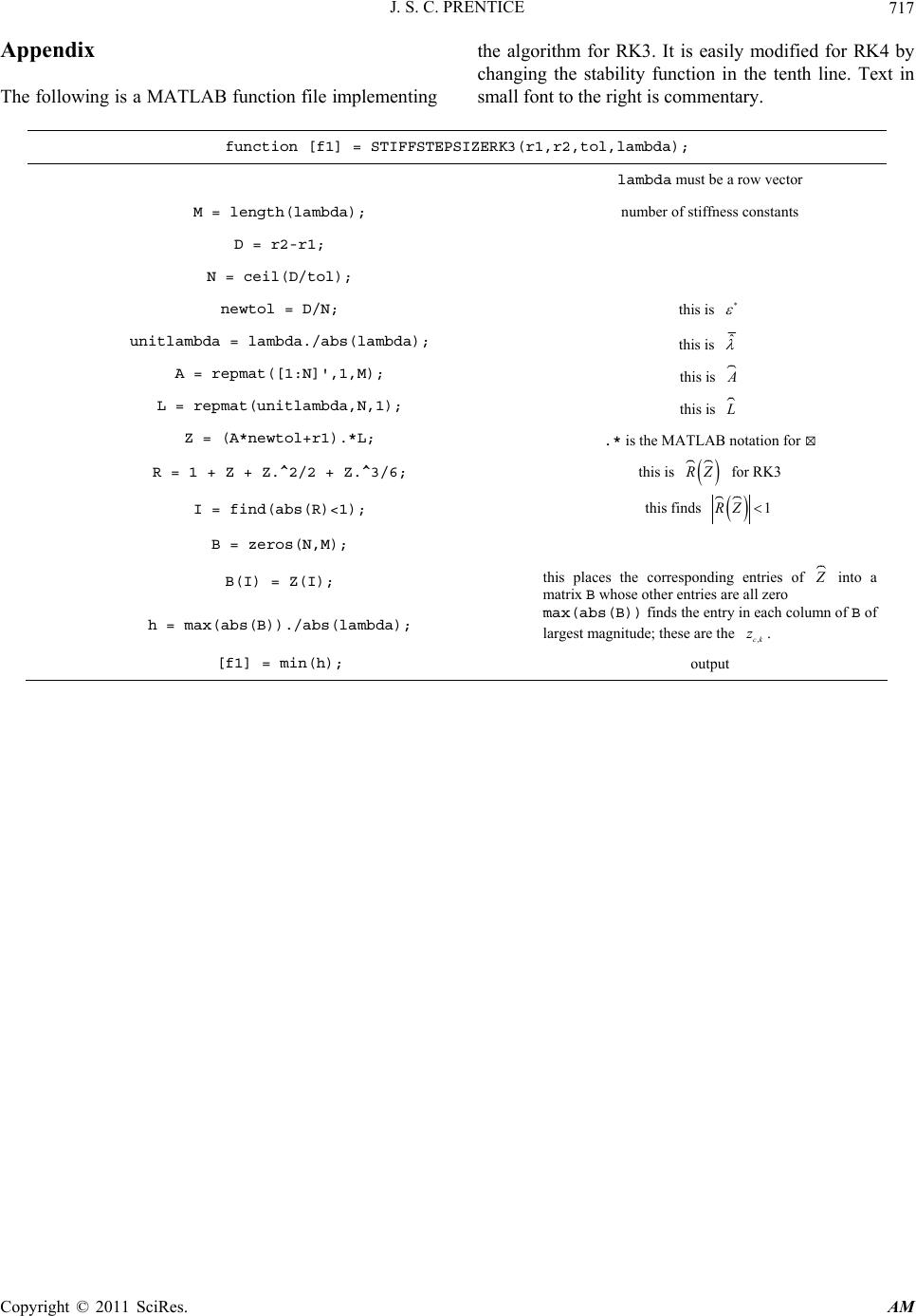

J. S. C. PRENTICE717
The following is a MATLAB function file implementing
r RK4 by
changing the stability function in the tenth line. Text in
small font to the right is commentary.
function [f1] = STIFFSTEPSIZERK3(r1,r2,tol,lambda);
Appendix the algorithm for RK3. It is easily modified fo
lambda must be a row vector
M = length(lambda); number of stiffness constants
D = r2-r1;
N = ceil(D/tol);
newtol = D/N; this is *

unitlambda = lambda./abs(lambda); this is ˆ

A = repmat([1:N]',1,M); this is
A

L = repmat(unitlambda,N,1); this is
L

Z = (A*newtol+r1).*L; .* is the MATLAB notation for ⊠
R = 1 + Z + Z.^2/2 + Z.^3/6; this is

R
Z

 for RK3
I = find(abs(R)<1); this finds

1RZ 
 
B = zeros(N,M);
B(I) = Z(I); this places the corresponding entries of
Z
 into a
matrix B whose other entries are all zero
h = max(abs(B))./abs(lambda); max(abs(B)) finds the entry in each column of B of
largest magnitude; these are the
[f1] = min(h); output
,ck z.